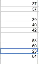
The following formula assumes your values are on column A (adjust all A:A references if they're not):
=Average(Filter(Sort(A:A;If(A:A="";0;Row(A:A));false);Row(A:A)<6))
To understand the formula above, paste its parts separately (when you get a part without the Filter formula, you'll need to wrap it on an ArrayFormula. e.g.
=Filter(Sort(A:A;If(A:A="";0;Row(A:A));false);Row(A:A)<6)
=ArrayFormula( Sort(A:A; If(A:A="";0;Row(A:A)); false) )
=ArrayFormula( Row(A:A) )
Place these "auxiliary" formulas on empty columns you might have on the sheet (in the first cells, e.g. D1, T1).
For non-entire columns, like you suggested, you may also need to wrap the whole formula in an array formula, e.g.
=ArrayFormula( Average(Filter(Sort(K1:K10;If(K1:K10="";0;Row(K1:K10));false);Row(K1:K10)<6)) )
I initially thought that Filter formula would behave like the ArrayFormula, but it seems it does not "recursion" down to the inners of its parameters. Hance, the ArrayFormula is required for the IF to work properly. I do not know why it did work for A:A though.

