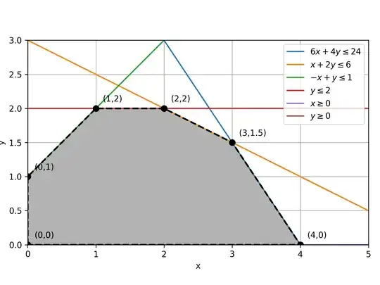
Here is a graphical representation of the problem, inspired from How to visualize feasible region for linear programming (with arbitrary inequalities) in Numpy/MatplotLib?
import numpy as np
import matplotlib.pyplot as plt

m = np.linspace(0,5,200)
x,y = np.meshgrid(m,m)
plt.imshow(((6*x+4*y<=24)&(x+2*y<=6)&(-x+y<=1)&(y<=2)&(x>=0)&(y>=0)).astype(int),
    extent=(x.min(),x.max(),y.min(),y.max()),origin='lower',cmap='Greys',alpha=0.3);
# plot constraints
x = np.linspace(0, 5, 2000)
# 6*x+4*y<=24
y0 = 6-1.5*x
# x+2*y<=6
y1 = 3-0.5*x
# -x+y<=1
y2 = 1+x
# y <= 2
y3 = (x*0) + 2
# x >= 0
y4 = x*0
plt.plot(x, y0, label=r'$6x+4y\leq24$')
plt.plot(x, y1, label=r'$x+2y\leq6$')
plt.plot(x, y2, label=r'$-x+y\leq1$')
plt.plot(x, 2*np.ones_like(x), label=r'$y\leq2$')
plt.plot(x, y4, label=r'$x\geq0$')
plt.plot([0,0],[0,3], label=r'$y\geq0$')
xv = [0,0,1,2,3,4,0]; yv = [0,1,2,2,1.5,0,0]
plt.plot(xv,yv,'ko--',markersize=7,linewidth=2)
for i in range(len(xv)):
    plt.text(xv[i]+0.1,yv[i]+0.1,f'({xv[i]},{yv[i]})')
plt.xlim(0,5); plt.ylim(0,3); plt.grid(); plt.tight_layout()
plt.legend(loc=1); plt.xlabel('x'); plt.ylabel('y')
plt.show()
The problem is missing an objective function so any of the shaded points satisfy the inequalities. If it did have an objective function (e.g. Maximize x+y) then many capable Python solvers can handle this problem. Here is a Linear Programming example in GEKKO that also supports mixed integer, nonlinear, and differential constraints.
from gekko import GEKKO
m = GEKKO(remote=False)
x,y = m.Array(m.Var,2,lb=0)
m.Equations([6*x+4*y<=24,x+2*y<=6,-x+y<=1,y<=2])
m.Maximize(x+y)
m.solve(disp=False)
Large scale LP problems are solved in matrix form or in sparse matrix form where only the non-zeros of the matrices are stored. There is a tutorial on LP solutions with a few examples that I developed for a university course.
 .
.