ggplot2 + gridExtra: how to ensure geom_bar in different size plot grobs result in exact same bar width

Question

This question is motivated by further exploring this question. The problem with the accepted solution becomes more obvious when there is a greater disparity in the number of bars per facet. Take a look at this data and the resultant plot using that solution:

# create slightly contrived data to better highlight width problems
data <- data.frame(ID=factor(c(rep(1,9), rep(2,6), rep(3,6), rep(4,3), rep(5,3))),
                   TYPE=factor(rep(1:3,length(ID)/3)),
                   TIME=factor(c(1,1,1,2,2,2,3,3,3,1,1,1,2,2,2,1,1,1,2,2,2,1,1,1,1,1,1)),
                   VAL=runif(27))

# implement previously suggested solution
base.width <- 0.9
data$w <- base.width
# facet two has 3 bars compared to facet one's 5 bars
data$w[data$TIME==2] <- base.width * 3/5
# facet 3 has 1 bar compared to facet one's 5 bars
data$w[data$TIME==3] <- base.width * 1/5
ggplot(data, aes(x=ID, y=VAL, fill=TYPE)) +
  facet_wrap(~TIME, ncol=1, scale="free") +
  geom_bar(position="stack", aes(width = w),stat = "identity") +
  coord_flip()

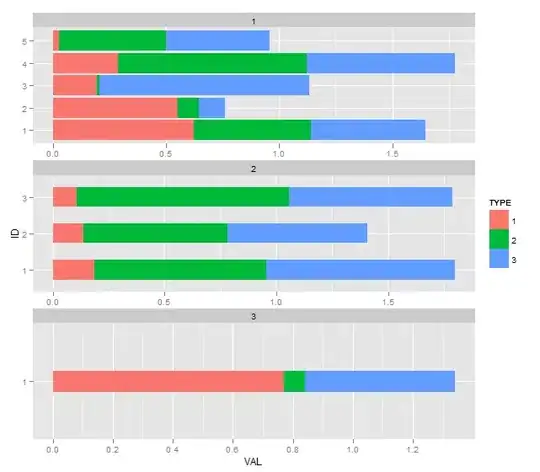
You'll notice the widths look exactly right, but the whitespace in facet 3 is quite glaring. There is no easy way to fix this in ggplot2 that I have seen yet (facet_wrap does not have a space option).

Next step is to try to solve this using gridExtra:

# create each of the three plots, don't worry about legend for now
p1 <- ggplot(data[data$TIME==1,], aes(x=ID, y=VAL, fill=TYPE)) +
  facet_wrap(~ TIME, ncol=1) +
  geom_bar(position="stack", show_guide=FALSE) +
  coord_flip()
p2 <- ggplot(data[data$TIME==2,], aes(x=ID, y=VAL, fill=TYPE)) +
  facet_wrap(~ TIME, ncol=1) +
  geom_bar(position="stack", show_guide=FALSE) +
  coord_flip()
p3 <- ggplot(data[data$TIME==3,], aes(x=ID, y=VAL, fill=TYPE)) +
  facet_wrap(~ TIME, ncol=1) +
  geom_bar(position="stack", show_guide=FALSE) +
  coord_flip()

# use similar arithmetic to try and get layout correct
require(gridExtra)
heights <- c(5, 3, 1) / sum(5, 3, 1)
print(arrangeGrob(p1 ,p2, p3, ncol=1,
            heights=heights))

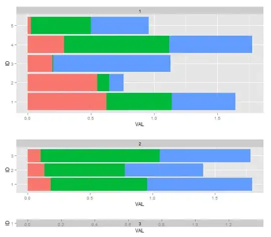
You'll notice I used the same arithmetic previously suggested based off the number of bars per facet, but in this case it ends up horribly wrong. This seems to be because there are extra "constant height" elements that I need to take into consideration in the math.

Another complication (I believe) is that the final output (and whether or not the widths match) will also depend on the width and height of where I'm outputting the final grob to, whether its in a R/RStudio environment, or to a PNG file.

How can I accomplish this?

Answer 1

Something like this appear to work, but it doesn't - not completely. It has the appearance of working because the levels of the ID factor are sequential. Anything else, and scale = "free" fails. But it might be possible to develop further. The method uses facet_grid, and thus space = "free" can be used. The method uses geom_rect to layer differently coloured rectangles on top of each other. It needs cumulative sums to be calculated so that the right-hand edge of each rectangle can be positioned.

data <- data.frame(ID=factor(c(rep(1,9), rep(2,6), rep(3,6), rep(4,3), rep(5,3))),
                   TYPE=factor(rep(1:3,3)),
                   TIME=factor(c(1,1,1,2,2,2,3,3,3,1,1,1,2,2,2,1,1,1,2,2,2,1,1,1,1,1,1)),
                   VAL=runif(27))

library(ggplot2)
library(plyr)

# Get the cumulative sums
data = ddply(data, .(ID, TIME), mutate, CUMSUMVAL = cumsum(VAL))

ggplot(data, aes(x=VAL, y = as.numeric(ID), fill=TYPE)) +
   geom_rect(data = subset(data, TYPE == 3), aes(xmin = 0, xmax = CUMSUMVAL, ymin = as.numeric(ID)-.2, ymax = as.numeric(ID)+.2)) +
   geom_rect(data = subset(data, TYPE == 2), aes(xmin = 0, xmax = CUMSUMVAL, ymin = as.numeric(ID)-.2, ymax = as.numeric(ID)+.2)) +
   geom_rect(data = subset(data, TYPE == 1), aes(xmin = 0, xmax = CUMSUMVAL, ymin = as.numeric(ID)-.2, ymax = as.numeric(ID)+.2)) +
   facet_grid(TIME~., space = "free", scale="free") +
   scale_y_continuous(breaks = c(1:5), expand = c(0, 0.2))

EDIT: OR really thick lines work a little better (I think)

ggplot(data, aes(x=VAL, y = ID, colour=TYPE)) +
       geom_segment(data = subset(data, TYPE == 3), aes(x = 0, xend = CUMSUMVAL, y = ID, yend = ID), size = 10) +
       geom_segment(data = subset(data, TYPE == 2), aes(x = 0, xend = CUMSUMVAL, y = ID, yend = ID), size = 10) +
       geom_segment(data = subset(data, TYPE == 1), aes(x = 0, xend = CUMSUMVAL, y = ID, yend = ID), size = 10) +
       facet_grid(TIME~., space = "free", scale="free") 

Additional Edit Taking the data from your earleir post, and modifying it a little.
Updated opts is deprecated; using theme instead.

df <- structure(list(ID = structure(c(1L, 1L, 1L, 1L, 1L, 2L, 2L, 2L, 
2L, 2L, 2L, 3L, 3L, 3L, 3L, 3L, 3L, 4L, 4L, 4L, 4L, 4L, 4L, 5L, 
5L, 5L, 5L, 5L, 5L, 6L, 6L, 6L, 6L, 6L, 6L, 7L, 7L, 7L), .Label = c("a", 
"b", "c", "d", "e", "f", "g"), class = "factor"), TYPE = structure(c(1L, 
2L, 3L, 4L, 5L, 1L, 2L, 3L, 4L, 5L, 6L, 1L, 2L, 3L, 4L, 5L, 6L, 
1L, 2L, 3L, 4L, 5L, 6L, 1L, 2L, 3L, 4L, 5L, 6L, 1L, 2L, 3L, 4L, 
5L, 6L, 1L, 2L, 3L), .Label = c("1", "2", "3", "4", "5", "6", 
"7", "8"), class = "factor"), TIME = structure(c(2L, 2L, 2L, 
2L, 2L, 1L, 1L, 1L, 1L, 1L, 1L, 1L, 1L, 1L, 1L, 1L, 1L, 2L, 2L, 
2L, 2L, 2L, 2L, 1L, 1L, 1L, 1L, 1L, 1L, 3L, 3L, 3L, 3L, 3L, 3L, 
1L, 1L, 1L), .Label = c("One", "Five", "Fifteen"), class = "factor"), VAL = c(0.937377670081332, 
0.522220720537007, 0.278690102742985, 0.967633064137772, 0.116124767344445, 
0.0544306698720902, 0.470229141646996, 0.62017166428268, 0.195459847105667, 
0.732876230962574, 0.996336271753535, 0.983087373664603, 0.666449476964772, 
0.291554537601769, 0.167933790013194, 0.860138458199799, 0.172361251665279, 
0.833266809117049, 0.620465772924945, 0.786503327777609, 0.761877260869369, 
0.425386636285111, 0.612077651312575, 0.178726130630821, 0.528709076810628, 
0.492527724476531, 0.472576208412647, 0.0702785139437765, 0.696220921119675, 
0.230852259788662, 0.359884874196723, 0.518227979075164, 0.259466265095398, 
0.149970305617899, 0.00682218233123422, 0.463400925742462, 0.924704828299582, 
0.229068386601284)), .Names = c("ID", "TYPE", "TIME", "VAL"), row.names = c(NA, 
-38L), class = "data.frame")

library(ggplot2)
library(plyr)

data = ddply(df, .(ID, TIME), mutate, CUMSUMVAL = cumsum(VAL))

ggplot(data, aes(x=VAL, y = ID, colour=TYPE)) +
           geom_segment(data = subset(data, TYPE == 6), aes(x = 0, xend = CUMSUMVAL, y = ID, yend = ID), size = 10) +
           geom_segment(data = subset(data, TYPE == 5), aes(x = 0, xend = CUMSUMVAL, y = ID, yend = ID), size = 10) +
           geom_segment(data = subset(data, TYPE == 4), aes(x = 0, xend = CUMSUMVAL, y = ID, yend = ID), size = 10) +
           geom_segment(data = subset(data, TYPE == 3), aes(x = 0, xend = CUMSUMVAL, y = ID, yend = ID), size = 10) +
           geom_segment(data = subset(data, TYPE == 2), aes(x = 0, xend = CUMSUMVAL, y = ID, yend = ID), size = 10) +
           geom_segment(data = subset(data, TYPE == 1), aes(x = 0, xend = CUMSUMVAL, y = ID, yend = ID), size = 10) +
           facet_grid(TIME~., space = "free", scale="free") +
           theme(strip.text.y = element_text(angle = 0))

Answer 2

Changing the gtable doesn't help, unfortunately, as the bar width is in relative units,

g = ggplot_gtable(ggplot_build(p))
panels = which(sapply(g$heights, attr, "unit") == "null")
g$heights[[panels[1]]] <- unit(5, "null")
g$heights[[panels[2]]] <- unit(3, "null")
g$heights[[panels[3]]] <- unit(1, "null")
grid.draw(g)