Get the minimal surface solution of a 3D contour

Question

I have a set of 3D points defining a 3D contour.

What I want to do is to obtain the minimal surface representation corresponding to this contour (see Minimal Surfaces in Wikipedia). Basically, this requires to solve a nonlinear partial differential equation.

In Matlab, this is almost straightforward using the pdenonlinfunction (see Matlab's documentation). An example of its usage for solving a minimal surface problem can be found here: Minimal Surface Problem on the Unit Disk.

I need to make such an implementation in Python, but up to know I haven't found any web resources on how to do this.

Can anyone point me any resources/examples of such implementation?

Thanks, Miguel.

---

UPDATE

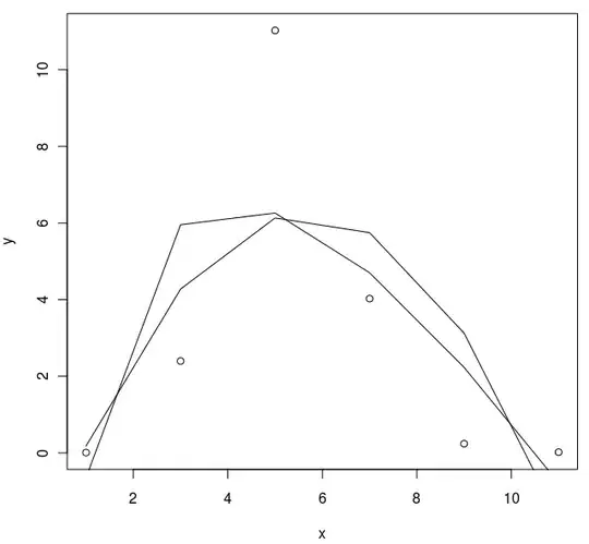
The 3D surface (ideally a triangular mesh representation) I want to find is bounded by this set of 3D points (as seen in this figure, the points lie in the best-fit plane):

Ok, so doing some research I found that this minimal surface problem is related with the solution of the Biharmonic Equation, and I also found that the Thin-plate spline is the fundamental solution to this equation.

So I think the approach would be to try to fit this sparse representation of the surface (given by the 3D contour of points) using thin-plate splines. I found this example in scipy.interpolate where scattered data (x,y,z format) is interpolated using thin-plate splines to obtain the ZI coordinates on a uniform grid (XI,YI).

Two questions arise:

1. Would thin-plate spline interpolation be the correct approach for the problem of computing the surface from the set of 3D contour points?
2. If so, how to perform thin-plate interpolation on scipy with a NON-UNIFORM grid?

Thanks again! Miguel

---

UPDATE: IMPLEMENTATION IN MATLAB (BUT IT DOESN'T WORK ON SCIPY PYTHON)

I followed this example using Matlab's tpaps function and obtained the minimal surface fitted to my contour on a uniform grid. This is the result in Matlab (looks great!):

However I need to implement this in Python, so I'm using the package scipy.interpolate.Rbf and the thin-plate function. Here's the code in python (XYZ contains the 3D coordinates of each point in the contour):

GRID_POINTS = 25
x_min = XYZ[:,0].min()
x_max = XYZ[:,0].max()
y_min = XYZ[:,1].min()
y_max = XYZ[:,1].max()
xi = np.linspace(x_min, x_max, GRID_POINTS)
yi = np.linspace(y_min, y_max, GRID_POINTS)
XI, YI = np.meshgrid(xi, yi)

from scipy.interpolate import Rbf
rbf = Rbf(XYZ[:,0],XYZ[:,1],XYZ[:,2],function='thin-plate',smooth=0.0)
ZI = rbf(XI,YI)

However this is the result (quite different from that obtained in Matlab):

It's evident that scipy's result does not correspond to a minimal surface.

Is scipy.interpolate.Rbf + thin-plate doing as expected, why does it differ from Matlab's result?

Answer 1

You can use FEniCS:

from fenics import (
    UnitSquareMesh,
    FunctionSpace,
    Expression,
    interpolate,
    assemble,
    sqrt,
    inner,
    grad,
    dx,
    TrialFunction,
    TestFunction,
    Function,
    solve,
    DirichletBC,
    DomainBoundary,
    MPI,
    XDMFFile,
)

# Create mesh and define function space
mesh = UnitSquareMesh(100, 100)
V = FunctionSpace(mesh, "Lagrange", 2)

# initial guess (its boundary values specify the Dirichlet boundary conditions)
# (larger coefficient in front of the sin term makes the problem "more nonlinear")
u0 = Expression("a*sin(2.5*pi*x[1])*x[0]", a=0.2, degree=5)
u = interpolate(u0, V)
print(
    "initial surface area: {}".format(assemble(sqrt(1 + inner(grad(u), grad(u))) * dx))
)

# Define the linearized weak formulation for the Newton iteration
du = TrialFunction(V)
v = TestFunction(V)
q = (1 + inner(grad(u), grad(u))) ** (-0.5)
a = (
    q * inner(grad(du), grad(v)) * dx
    - q ** 3 * inner(grad(u), grad(du)) * inner(grad(u), grad(v)) * dx
)
L = -q * inner(grad(u), grad(v)) * dx
du = Function(V)

# Newton iteration
tol = 1.0e-5
maxiter = 30
for iter in range(maxiter):
    # compute the Newton increment by solving the linearized problem;
    # note that the increment has *homogeneous* Dirichlet boundary conditions
    solve(a == L, du, DirichletBC(V, 0.0, DomainBoundary()))
    u.vector()[:] += du.vector()  # update the solution
    eps = sqrt(
        abs(assemble(inner(grad(du), grad(du)) * dx))
    )  # check increment size as convergence test
    area = assemble(sqrt(1 + inner(grad(u), grad(u))) * dx)
    print(
        f"iteration{iter + 1:3d}  H1 seminorm of delta: {eps:10.2e}  area: {area:13.5e}"
    )
    if eps < tol:
        break

if eps > tol:
    print("no convergence after {} Newton iterations".format(iter + 1))
else:
    print("convergence after {} Newton iterations".format(iter + 1))

with XDMFFile(MPI.comm_world, "out.xdmf") as xdmf_file:
    xdmf_file.write(u)

(Modified from http://www-users.math.umn.edu/~arnold/8445/programs/minimalsurf-newton.py.)

Answer 2

Obviously Matlab and SciPy understand TPS in different ways. The Matlab implementation looks correct. SciPy treats TPS the same way as others RBFs, so you could implement it correctly in Python yourself - it would be enough to form a matrix of the related linear equation system and solve it to receive TPS' coefficients.