49

I've been looking around in Numpy/Scipy for modules containing finite difference functions. However, the closest thing I've found is numpy.gradient(), which is good for 1st-order finite differences of 2nd order accuracy, but not so much if you're wanting higher-order derivatives or more accurate methods. I haven't even found very many specific modules for this sort of thing; most people seem to be doing a "roll-your-own" thing as they need them. So my question is if anyone knows of any modules (either part of Numpy/Scipy or a third-party module) that are specifically dedicated to higher-order (both in accuracy and derivative) finite difference methods. I've got my own code that I'm working on, but it's currently kind of slow, and I'm not going to attempt to optimize it if there's something already available.

Note that I am talking about finite differences, not derivatives. I've seen both scipy.misc.derivative() and Numdifftools, which take the derivative of an analytical function, which I don't have.

Tim Supinie
  • 983
  • 1
  • 9
  • 9
  • 2
    Would interpolating the data and then using `scipy.misc.derivative` on the interpolation function work for you? – unutbu Sep 24 '13 at 21:03
  • 3
    Take a look at `numpy.diff` (http://docs.scipy.org/doc/numpy/reference/generated/numpy.diff.html). – Warren Weckesser Sep 24 '13 at 21:26
  • 1
    Also, if your data is periodic, there is `scipy.fftpack.diff` (http://docs.scipy.org/doc/scipy/reference/generated/scipy.fftpack.diff.html). There is an example of its use here: http://wiki.scipy.org/Cookbook/KdV – Warren Weckesser Sep 24 '13 at 21:32
  • @unutbu: I guess in theory it could work, if I'm reading the documentation correctly, by setting the dx parameter to be the same as the grid spacing and forcing x0 to be at one of the grid points. However, my intent is to use this for 2- and 3- dimensional arrays, so for an MxNxP array, I'd have to create NxP interp1d objects for a derivative in the M direction, which seems a little slow. It would also require a Python loop, which I'd like to avoid, for the same reason. – Tim Supinie Sep 24 '13 at 21:32
  • @WarrenWeckesser: The data will not be periodic, in general. I hadn't found `numpy.diff` (somehow), but that looks like it only does 1st-order accuracy (forward- or backward-differencing). – Tim Supinie Sep 24 '13 at 21:39
  • @Tim What exactly do you mean by "1st-order _accuracy_"? – askewchan Sep 24 '13 at 21:53
  • 3
    @askewchan: Accuracy here refers to error in the finite difference approximation resulting from the truncation of the Taylor series. More accurate finite difference methods keep around more terms of the Taylor series, and are therefore closer to the true derivative at that point. 1st order keeps around fewer terms than 2nd order, and so on. – Tim Supinie Sep 24 '13 at 22:18
  • OK I'm not sure I understand how you can have a taylor series for a numerical array where each coefficient has more than one order of accuracy, but this probably isn't the place to try to learn it :P Have you tried convolving with the nth derivative of a gaussian? – askewchan Sep 24 '13 at 22:21
  • I should have said the Taylor series is used in the derivation of the approximation. I am unfamiliar with the convolving with a nth derivative of a Gaussian method, though, can you provide any additional information? – Tim Supinie Sep 24 '13 at 22:26

5 Answers5

59

One way to do this quickly is by convolution with the derivative of a gaussian kernel. The simple case is a convolution of your array with [-1, 1] which gives exactly the simple finite difference formula. Beyond that, (f*g)'= f'*g = f*g' where the * is convolution, so you end up with your derivative convolved with a plain gaussian, so of course this will smooth your data a bit, which can be minimized by choosing the smallest reasonable kernel.

import numpy as np
from scipy import ndimage
import matplotlib.pyplot as plt

#Data:
x = np.linspace(0,2*np.pi,100)
f = np.sin(x) + .02*(np.random.rand(100)-.5)

#Normalization:
dx = x[1] - x[0] # use np.diff(x) if x is not uniform
dxdx = dx**2

#First derivatives:
df = np.diff(f) / dx
cf = np.convolve(f, [1,-1]) / dx
gf = ndimage.gaussian_filter1d(f, sigma=1, order=1, mode='wrap') / dx

#Second derivatives:
ddf = np.diff(f, 2) / dxdx
ccf = np.convolve(f, [1, -2, 1]) / dxdx
ggf = ndimage.gaussian_filter1d(f, sigma=1, order=2, mode='wrap') / dxdx

#Plotting:
plt.figure()
plt.plot(x, f, 'k', lw=2, label='original')
plt.plot(x[:-1], df, 'r.', label='np.diff, 1')
plt.plot(x, cf[:-1], 'r--', label='np.convolve, [1,-1]')
plt.plot(x, gf, 'r', label='gaussian, 1')
plt.plot(x[:-2], ddf, 'g.', label='np.diff, 2')
plt.plot(x, ccf[:-2], 'g--', label='np.convolve, [1,-2,1]')
plt.plot(x, ggf, 'g', label='gaussian, 2')

derivatives

Since you mentioned np.gradient I assumed you had at least 2d arrays, so the following applies to that: This is built into the scipy.ndimage package if you want to do it for ndarrays. Be cautious though, because of course this doesn't give you the full gradient but I believe the product of all directions. Someone with better expertise will hopefully speak up.

Here's an example:

from scipy import ndimage

x = np.linspace(0,2*np.pi,100)
sine = np.sin(x)

im = sine * sine[...,None]
d1 = ndimage.gaussian_filter(im, sigma=5, order=1, mode='wrap')
d2 = ndimage.gaussian_filter(im, sigma=5, order=2, mode='wrap')

plt.figure()

plt.subplot(131)
plt.imshow(im)
plt.title('original')

plt.subplot(132)
plt.imshow(d1)
plt.title('first derivative')

plt.subplot(133)
plt.imshow(d2)
plt.title('second derivative')

2d-derivatives

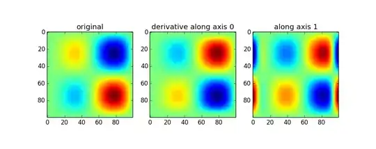
Use of the gaussian_filter1d allows you to take a directional derivative along a certain axis:

imx = im * x
d2_0 = ndimage.gaussian_filter1d(imx, axis=0, sigma=5, order=2, mode='wrap')
d2_1 = ndimage.gaussian_filter1d(imx, axis=1, sigma=5, order=2, mode='wrap')

plt.figure()
plt.subplot(131)
plt.imshow(imx)
plt.title('original')
plt.subplot(132)
plt.imshow(d2_0)
plt.title('derivative along axis 0')
plt.subplot(133)
plt.imshow(d2_1)
plt.title('along axis 1')

1d filter derivatives

The first set of results above are a little confusing to me (peaks in the original show up as peaks in the second derivative when the curvature should point down). Without looking further into how the 2d version works, I can only really recomend the 1d version. If you want the magnitude, simply do something like:

d2_mag = np.sqrt(d2_0**2 + d2_1**2)
askewchan
  • 45,161
  • 17
  • 118
  • 134
11

Definitely like the answer given by askewchan. This is a great technique. However, if you need to use numpy.convolve I wanted to offer this one little fix. Instead of doing:

#First derivatives:
cf = np.convolve(f, [1,-1]) / dx
....
#Second derivatives:
ccf = np.convolve(f, [1, -2, 1]) / dxdx
...
plt.plot(x, cf[:-1], 'r--', label='np.convolve, [1,-1]')
plt.plot(x, ccf[:-2], 'g--', label='np.convolve, [1,-2,1]')

...use the 'same' option in numpy.convolve like this:

#First derivatives:
cf = np.convolve(f, [1,-1],'same') / dx
...
#Second derivatives:
ccf = np.convolve(f, [1, -2, 1],'same') / dxdx
...
plt.plot(x, cf, 'rx', label='np.convolve, [1,-1]')
plt.plot(x, ccf, 'gx', label='np.convolve, [1,-2,1]')

...to avoid off-by-one index errors.

Also be careful about the x-index when plotting. The points from the numy.diff and numpy.convolve must be the same! To fix the off-by-one errors (using my 'same' code) use:

plt.plot(x, f, 'k', lw=2, label='original')
plt.plot(x[1:], df, 'r.', label='np.diff, 1')
plt.plot(x, cf, 'rx', label='np.convolve, [1,-1]')
plt.plot(x, gf, 'r', label='gaussian, 1')
plt.plot(x[1:-1], ddf, 'g.', label='np.diff, 2')
plt.plot(x, ccf, 'gx', label='np.convolve, [1,-2,1]')
plt.plot(x, ggf, 'g', label='gaussian, 2')

The points from the <code>numy.diff</code> and <code>numpy.convolve</code> must be the same!

Edit corrected auto-complete with s/bot/by/g

Kevin Johnson
  • 593
  • 4
  • 9
10

You may want to take a look at the findiff project. I have tried it out myself and it let's you conveniently take derivatives of numpy arrays of any dimension, any derivative order and any desired accuracy order. The project website says that it features:

  • Differentiate arrays of any number of dimensions along any axis
  • Partial derivatives of any desired order
  • Standard operators from vector calculus like gradient, divergence and curl
  • Can handle uniform and non-uniform grids
  • Can handle arbitrary linear combinations of derivatives with constant and variable coefficients
  • Accuracy order can be specified
  • Fully vectorized for speed
  • Calculate raw finite difference coefficients for any order and accuracy for uniform and non-uniform grids
owelk
  • 176
  • 1
  • 3
6

Another approach is to differentiate an interpolation of the data. This was suggested by unutbu, but I did not see the method used here or in any of the linked questions. UnivariateSpline, for example, from scipy.interpolate has a useful built-in derivative method.

import numpy as np
from scipy.interpolate import UnivariateSpline
import matplotlib.pyplot as plt

# data
n = 1000
x = np.linspace(0, 100, n)
y = 0.5 * np.cumsum(np.random.randn(n))

k = 5 # 5th degree spline
s = n - np.sqrt(2*n) # smoothing factor
spline_0 = UnivariateSpline(x, y, k=k, s=s)
spline_1 = UnivariateSpline(x, y, k=k, s=s).derivative(n=1)
spline_2 = UnivariateSpline(x, y, k=k, s=s).derivative(n=2)

# plot data, spline fit, and derivatives
fig = plt.figure()
ax = fig.add_subplot(111)

ax.plot(x, y, 'ko', ms=2, label='data')
ax.plot(x, spline_0(x), 'k', label='5th deg spline')
ax.plot(x, spline_1(x), 'r', label='1st order derivative')
ax.plot(x, spline_2(x), 'g', label='2nd order derivative')

ax.legend(loc='best')
ax.grid()

Note the zero-crossings of the first derivative (red curve) at the peaks and troughs of the spline fit (black curve).

enter image description here

lanery
  • 5,222
  • 3
  • 29
  • 43
  • Keep in mind that with `UnivariateSpline` you are limited to a fifth degree spline (`k<=5`), which means you are limited to `n=4` derivatives. Also, as is the case with Gaussian convolution, the smoothing factor will need to be changed as necessary. – lanery Apr 30 '16 at 07:44
2

FastFD can help:

pip install fastfd

basic documentation is found here:

https://github.com/stefanmeili/FastFD

and here:

https://github.com/stefanmeili/FastFD/tree/main/docs/examples