5

Basically I am trying to use the conditional formatting icon set that is a green dot, orange dot and red dot.

If my value is smaller than my formulas value, display the green dot.

If my value is equal to my formulas value, display the orange dot.

If my value is more than my formulas value, display the red dot.

This is the EXACT formula I am trying to use:

VLOOKUP(product_ID,product_db,3,FALSE)

product_ID is the cell next to the cell I am trying to apply the conditional formatting to. product_db is a large table within another worksheet.

Although, when I am trying to use this, the formatting is not applied to my cell at all. No dots are displayed.

I believe it is because of my formula. Any ideas?


EDIT:

Here are some screen shots of what is happening:

Here is the quantity before the conditioning:
Here is the conditioning with the formula being: =VLOOKUP(invoice_product,PRODUCT_DATABASE,3,FALSE)

enter image description here

The quantity is then the EXACT same as the first image, unchanged. The value that my formula should return is 2, hence the orange dot should be displayed.
Siddharth Rout
  • 147,039
  • 17
  • 206
  • 250
Fizzix
  • 23,679
  • 38
  • 110
  • 176
  • Since this is really about standard Excel features, I think this would be more appropriate to ask at [SuperUser](http://superuser.com/). See [this discussion](http://meta.stackexchange.com/questions/22922/which-site-do-excel-or-other-spreadsheet-formulas-belong-on) for some rationale. – Jonathon Reinhart Nov 15 '13 at 07:51
  • Did you put an `=` before the formula? – James L. Nov 15 '13 at 07:53
  • @JamesL. - Tried with and without the `=`, although still no luck. My VLOOKUP function is definitely correct since I have tried it out in a blank cell and it is returning the correct value. – Fizzix Nov 15 '13 at 07:57
  • 1
    @JonathonReinhart: That's an old thread. The current one now suggests that it can remain in SO. See [THIS](http://meta.stackexchange.com/questions/199823/slight-amendment-to-close-reason) – Siddharth Rout Nov 15 '13 at 08:03
  • @SiddharthRout Fair enough. I'm actually interested in the OP's question, but if it were me asking, I would still have asked at SU. Especially considering the conditional formatting is really what's at question here. – Jonathon Reinhart Nov 15 '13 at 08:07
  • @JonathonReinhart: True but since the OP is using formulas in conditional formatting and community thinks that formula is "Code" what can I say? Damn! I got heavily down voted for that :P – Siddharth Rout Nov 15 '13 at 08:08
  • @fizzix: Can you show us an example screenshot? – Siddharth Rout Nov 15 '13 at 08:09
  • @SiddharthRout I'm just saying, one `VLOOKUP()` doesn't make this much more of a programming question than including the word `"if"` in a sentence. The real question here is about getting conditional formatting working (which in this case uses formulas). I've retracted my close vote, but I still think it would be more beneficial for the OP and the community at SU. – Jonathon Reinhart Nov 15 '13 at 08:12
  • @SiddharthRout - Added an edit to my question with some more details. – Fizzix Nov 15 '13 at 08:19
  • @fizzix - What is the range that the conditional formatting rule is applied to? Does it include the cell with the value `2` in it (in the **Quantity** column)? – James L. Nov 15 '13 at 08:22
  • @fizzix: you are using Excel 2011? – Siddharth Rout Nov 15 '13 at 08:22
  • @SiddharthRout - Yes, Mac Excel 2011 – Fizzix Nov 15 '13 at 08:24
  • @JamesL. - The conditional formatting is only applied to the cell with the `2` in it, being the 'Quantity' column. The `invoice_product` is referring to the cell next to it which has the products ID. The VLOOKUP function should return the number `2` since the VLOOKUP is referring to another worksheet – Fizzix Nov 15 '13 at 08:26
  • @SiddharthRout - You may need to elaborate a little more. Not really to sure what you both mean. – Fizzix Nov 15 '13 at 08:27
  • I don't have MAC with me at the moment so I will use some screenshots from Excel 2010 to demonstrate what I mean.. Bare with me for few minutes – Siddharth Rout Nov 15 '13 at 08:28
  • @SiddharthRout - Thanks. Will stand by. – Fizzix Nov 15 '13 at 08:29
  • I created an example in Excel 2010 (Win) that approximates what you describe/show -- and it works. – James L. Nov 15 '13 at 08:32
  • @JamesL. - Anywhere that I could upload my file so that you could take a quick glance at it? – Fizzix Nov 15 '13 at 08:35
  • @fizzix - Sorry, I don't have a public location for file uploads. Take a look at my answer and see if there is perhaps something you need to tweak in your workbook. – James L. Nov 15 '13 at 08:53

1 Answers1

5

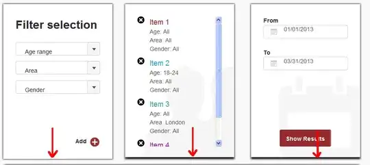
Your conditional formatting formula included a range for the first parameter of the VLOOKUP formula. You can't do that, it must be a single cell. You can use an INDIRECT function to resolve the cell to the immediate left of the one in the quantity column. Look at the following screen shot. Also, because you are using icons as the conditional formatting, you cannot apply it to a range, it must be a single cell for the INDIRECT function in the VLOOKUP formula to work. You could apply it to a range if you simply formatted the color of the text, but not when using icons. Follow the instructions in the image:

Image of Solution

James L.
  • 9,384
  • 5
  • 38
  • 77
  • I'll test mine out and then let you know how it goes. Thanks – Fizzix Nov 15 '13 at 08:53
  • 1
    Did you verify that the cell format for the cell with the `2` and the format of the value returned from the `VLOOKUP` function are the same format? – James L. Nov 16 '13 at 00:12
  • Worked perfectly! Thank you very much for your help, was very challenging haha :) – Fizzix Nov 17 '13 at 04:21