How to set uniform bar width in multi-histogram plot in R

Question

I am reading a dataset "Dummy_data.csv" with 26 columns and 4288 instances, where there are overall 17 parameters (columns) which are important for our data analysis. 6 out of 17 parameters i.e. (param1, param2, param3, param5, param6, param7) are critical parameters which being simultaneously out of range determines whether the item would be defective or not (class label). For example,

range1 = (min1, max1) = (0.25, 0.35)
range2 = (min2, max2) = (2.5, 3.1)
range3 = (min3, max3) = (680, 700)
range5 = (min5, max5) = (56, 64)
range6 = (min6, max6) = (40, 60)
range7 = (min7, max7) = (28, 38)

if (param1 out of range1 & param2 out of range2 & param3 out of range3 &
    param5 out of range5 & param6 out of range6 & param7 out of range7)
    class = 'defective'
else
    class = 'ok'

We need to do two defect analyses on the above data. First, I need to find out the % share of defects from the total number of items. Second, I need to find out the frequency histogram of the out of range values for each of the 6 critical parameters to have an understanding of which out-of-range values of these critical parameters contributed more to defective items.

What I did: Since the ranges of these 6 critical parameters were mostly non-overlapping, first I scaled the 17 parameters (though scaling the 6 critical parameters would have been sufficient!) using (x - min(x))/(max(x)-min(x))to an interval of (0, 1) so that I can do the frequency distribution of out of range values for 6 parameters on an uniform scale of x-axis. In graphical terms, this means a parameter value less than 0 means less than minimum value whereas a parameter value greater than 1 means more than maximum value. Thus, I filtered all the defective instances from the dataset in the z data frame and draw a pie chart to show percentage defective and OK items. (first analysis)

For the frequency histogram (second analysis), I filtered all the defective instances from the scaled dataset scaled.dat.df into defect.dat.df. Then I select the min and max from all the 6 parameters to determine the defect interval range. Next, I binned the unique values of each of the 6 parameters into p1.bin.defect.dat.df to p7.bin.defect.dat.df and plotted the individual histograms using the plot function on the same plot.

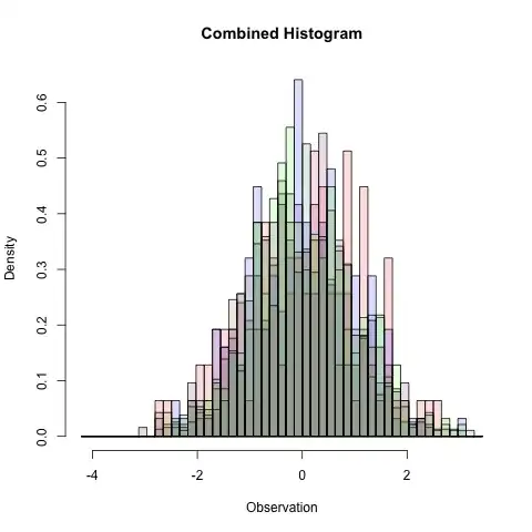
The problem with multiple overlapping histogram plots
I am getting the multi-histogram plot as shown below but the problem is that the width of the bars are varying for the 6 parameters. Does anybody have an idea of how to set a uniform bar width for a multi-histogram plot? Also, how can I add a suitable legend to this multi-hist plot ?

Any helpful suggestions/answers will be highly appreciated and rewarded accordingly.

Note: I followed the other thread on multiple histogram plot here how-to-plot-two-histograms-together-in-r and want a multi-hist plot very similar to this but 6 overlapping hist plots instead of 2 overlapping hist plots (as in the thread)

library(RWeka)
library(party)
library(plyr)
library(plotrix)
library(sm)

#read data and class labels
dat <- read.csv("Dummy_data.csv", head=T, sep=",")
datm <- as.matrix(dat[,8:24])
class <- as.matrix(dat[,26])

#center and scale data
center <- c(0.25, 2.5, 680, 1067, 56, 40, 28, -99, -99, 40, 5, 50, 5000, 15000, 11.3, 9.1, 0)
scale <- c(0.1, 0.6, 20, 6, 8, 20, 10, 19, 19, 20, 2, 10, 500, 1000, 3.4, 18.3, 5)
scaled.datm <- scale(datm, center, scale)
write.table(scaled.datm, 
file = "C:\\Users\\schakrabarti\\Documents\\Dummy_data_whdr17.csv", 
append=FALSE, quote=TRUE, sep=",", eol = "\n", na = "NA", dec = ".", 
row.names = FALSE, col.names = TRUE, qmethod = c("escape", "double"),
fileEncoding = "")

#filter total non-compliants
scaled.dat.df <- as.data.frame(scaled.datm)
total <- length(scaled.dat.df[,1])
z <- c((scaled.dat.df[,"PARAM1"]<0 | scaled.dat.df[,"PARAM1"]>1) & 
    (scaled.dat.df[,"PARAM2"]<0 | scaled.dat.df[,"PARAM2"]>1) & 
    (scaled.dat.df[,"PARAM3"]<0 | scaled.dat.df[,"PARAM3"]>1) & 
    (scaled.dat.df[,"PARAM5"]<0 | scaled.dat.df[,"PARAM5"]>1) &
    (scaled.dat.df[,"PARAM6"]<0 | scaled.dat.df[,"PARAM6"]>1) & 
    (scaled.dat.df[,"PARAM7"]<0 | scaled.dat.df[,"PARAM7"]>1) )
noncompliant <- length(z[z == TRUE])

slices <- c(noncompliant, total - noncompliant)
labls <- c("NOT OK","OK")
pct <- round(slices/sum(slices)*100, digits=2)
labls <- paste(labls, pct)
labls <- paste(labls, "%", sep="")

#pie3D(slices,labels=labls,explode=0.05, col=c(rgb(0.75,0,0.5),rgb(0,1,0.75)),main="Defect Analysis due to critical parameters")
pie(slices,labels=labls,main="Defect Analysis due to critical parameters")

#filter non-compliants due to individual params
defect.dat.df <- scaled.dat.df[z,]

#select defect interval range
min <- min(as.numeric(sapply(defect.dat.df[,c("PARAM1","PARAM2","PARAM3","PARAM5","PARAM6","PARAM7")], function(x) min(as.numeric(x)))))
max <- max(as.numeric(sapply(defect.dat.df[,c("PARAM1","PARAM2","PARAM3","PARAM5","PARAM6","PARAM7")], function(x) max(as.numeric(x)))))


#plot histogram for param1 defect
#p1.bin.defect.dat.df <- binning(defect.dat.df[,c("PARAM1")], breaks=seq(-0.4,0.2,by=0.2))
p1.bin.defect.dat.df <- binning(defect.dat.df[,c("PARAM1")], breaks=seq(min,max,by=0.2))
#h1 <- hist(defect.dat.df[,c("PARAM1")])
#plot(h1, col=rgb(1,0,0,1/7), xlab="Param Defect Intervals", main="Frequency of Parameter Defects", xlim=c(head(p1.bin.defect.dat.df$breaks, n=1),tail(p1.bin.defect.dat.df$breaks, n=1)))
h1 <- hist(defect.dat.df[,c("PARAM1")], col=rgb(1,0,0,1/7), xlab="Param Defect Intervals", main="Frequency of Parameter Defects", xlim=c(head(p1.bin.defect.dat.df$breaks, n=1),tail(p1.bin.defect.dat.df$breaks, n=1)))
#h1 <- hist(defect.dat.df[,c("PARAM1")], col=rgb(1,0,0,1/7), xlab="Param Defect Intervals", main="Frequency of Parameter Defects", xlim=c(min,max))
box()

p2.bin.defect.dat.df <- binning(defect.dat.df[,c("PARAM2")], breaks=seq(min,max,by=0.2))
#h2 <- hist(defect.dat.df[,c("PARAM2")])
#plot(h2, col=rgb(0,0,1,1/7), xlim=c(head(p1.bin.defect.dat.df$breaks, n=1),tail(p1.bin.defect.dat.df$breaks, n=1)))
h2 <- hist(defect.dat.df[,c("PARAM2")], col=rgb(0,0,1,1/7), xlab="Param Defect Intervals", main="Frequency of Parameter Defects", xlim=c(head(p2.bin.defect.dat.df$breaks, n=1),tail(p2.bin.defect.dat.df$breaks, n=1)), add=T)
#h2 <- hist(defect.dat.df[,c("PARAM2")], col=rgb(0,0,1,1/7), xlab="Param Defect Intervals", main="Frequency of Parameter Defects", xlim=c(min,max), add=T)
box()

p3.bin.defect.dat.df <- binning(defect.dat.df[,c("PARAM3")], breaks=seq(min,max,by=0.2))
#h3 <- hist(defect.dat.df[,c("PARAM3")])
#plot(h3, col=rgb(0,1,0,1/7), xlim=c(head(p1.bin.defect.dat.df$breaks, n=1),tail(p1.bin.defect.dat.df$breaks, n=1)))
h3 <- hist(defect.dat.df[,c("PARAM3")], col=rgb(0,1,0,1/7), xlab="Param Defect Intervals", main="Frequency of Parameter Defects", xlim=c(head(p3.bin.defect.dat.df$breaks, n=1),tail(p3.bin.defect.dat.df$breaks, n=1)), add=T)
#h3 <- hist(defect.dat.df[,c("PARAM3")], col=rgb(0,1,0,1/7), xlab="Param Defect Intervals", main="Frequency of Parameter Defects", xlim=c(min,max), add=T)
box()

p5.bin.defect.dat.df <- binning(defect.dat.df[,c("PARAM5")], breaks=seq(min,max,by=0.2))
#h5 <- hist(defect.dat.df[,c("PARAM5")])
#plot(h5, col=rgb(0.5,0.5,0,1/7), xlim=c(head(p1.bin.defect.dat.df$breaks, n=1),tail(p1.bin.defect.dat.df$breaks, n=1)))
h5 <- hist(defect.dat.df[,c("PARAM5")], col=rgb(0.5,0,0.5,1/7), xlab="Param Defect Intervals", main="Frequency of Parameter Defects", xlim=c(head(p5.bin.defect.dat.df$breaks, n=1),tail(p5.bin.defect.dat.df$breaks, n=1)), add=T)
#h5 <- hist(defect.dat.df[,c("PARAM5")], col=rgb(0.5,0,0.5,1/7), xlab="Param Defect Intervals", main="Frequency of Parameter Defects", xlim=c(min,max), add=T)
box()

p6.bin.defect.dat.df <- binning(defect.dat.df[,c("PARAM6")], breaks=seq(min,max,by=0.2))
#h6 <- hist(defect.dat.df[,c("PARAM6")])
#plot(h6, col=rgb(0,0.5,0.5,1/7), xlim=c(head(p1.bin.defect.dat.df$breaks, n=1),tail(p1.bin.defect.dat.df$breaks, n=1)))
h6 <- hist(defect.dat.df[,c("PARAM6")], col=rgb(0,0.5,0.5,1/7), xlab="Param Defect Intervals", main="Frequency of Parameter Defects", xlim=c(head(p6.bin.defect.dat.df$breaks, n=1),tail(p6.bin.defect.dat.df$breaks, n=1)), add=T)
#h6 <- hist(defect.dat.df[,c("PARAM6")], col=rgb(0,0.5,0.5,1/7), xlab="Param Defect Intervals", main="Frequency of Parameter Defects", xlim=c(min,max), add=T)
box()

p7.bin.defect.dat.df <- binning(defect.dat.df[,c("PARAM7")], breaks=seq(min,max,by=0.2))
#h7 <- hist(defect.dat.df[,c("PARAM7")])
#plot(h7, col=rgb(0.5,0,0.5,1/7), xlim=c(head(p1.bin.defect.dat.df$breaks, n=1),tail(p1.bin.defect.dat.df$breaks, n=1)))
h7 <- hist(defect.dat.df[,c("PARAM7")], col=rgb(0.5,0.5,0,1/7), xlab="Param Defect Intervals", main="Frequency of Parameter Defects", xlim=c(head(p7.bin.defect.dat.df$breaks, n=1),tail(p7.bin.defect.dat.df$breaks, n=1)), add=T)
#h7 <- hist(defect.dat.df[,c("PARAM7")], col=rgb(0.5,0.5,0,1/7), xlab="Param Defect Intervals", main="Frequency of Parameter Defects", xlim=c(min,max), add=T)
box()

enter image description here

Did you mean to tag this as [plotrix] rather than [ggplot2]? — MattLBeck, May 21 '14 at 15:18
yes something of that sort. I am trying multiple hist's with add=T — somnathchakrabarti, May 21 '14 at 15:20
I believe "bins" in the above answer example should = observations, and density should = counts. That's how I got this to work on my own data correctly. — John Clarke, Mar 31 '18 at 15:29

score 0 · Answer 1 · answered May 22 '14 at 05:29

Really, in order to get the bars the same width you want to use the same breaks across all the groups. I went ahead and created some sample data. Instead of having a bunch of different data.frames, I kept everything in lists.

#sample data
set.seed(15)
observations <- lapply(1:6, function(x) rnorm(100*x))

Here we have 6 items, each with a different number of random draws from a standard normal distribution. Now I'll rind the total range and make 50 breaks

maxrange <- range(sapply(observations, range))
breaks <- seq(maxrange[1], maxrange[2], length.out=50)

Now i'll apply these same breaks to all the sets and i'll calculate the histogram data without actually plotting it

hists <- lapply(bins, hist, breaks=breaks, plot=F)

To help with plotting i need to pre-calculate the the ylim to make sure the first plot is tall enough for all the data for all the other plots. I'll also set up the colors now.

ylim <- range(sapply(hists, function(x) {range(x$density)}))
cols<-list(
    rgb(1,0,0,1/7), rgb(0,0,1,1/7), rgb(0,1,0,1/7),
    rgb(0.5,0,0.5,1/7), rgb(0,0.5,0.5,1/7), rgb(0.5,0.5,0,1/7)
)

Now we plot the first histogram with all the labels and such we want, then we plot all the others on top

plot(hists[[1]], ylim=ylim, col=cols[[1]], freq=F, 
    main="Combined Histogram", xlab="Observation")
invisible(mapply(function(x, c) 
    plot(x, ylim=ylim, col=c, freq=F, add=T), 
hists[-1], cols[-1]))

multiple histogram

How to set uniform bar width in multi-histogram plot in R

1 Answers1