2

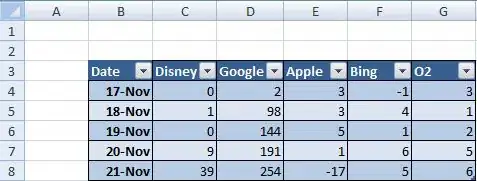
I have an Excel table of the following format:

enter image description here

And I would like to answer the following question using Excel formulae:

  • What is the sum for Disney during 17-Nov until 20-Nov?

My attempts I tried the following approaches, unsuccessfully:

  1. Using SUMIFS with an array:

    =SUMIFS(c4:g8,c3:g3,i1,b4:b8,">="&i2,b4:b8,"<="&i3)

where i1 contains Disney, i2 contains 17-Nov in the date format, and i3 contains 20-Nov in the date format.

But this doesn't work because we are submitting an array where we must specify a range of cells. So I tried the following method:

  1. Using SUMIFS with a range:

    =SUMIFS(c4:g8,b4:b8,">="&i2,b4:b8,"<="&i3)

But this doesn't work either, since I think we are using the >, < operators for text (the date values in the table).

So, what to do?
Should I change the format of the table completely?
Should I convert it back to range?

pnuts
  • 58,317
  • 11
  • 87
  • 139
info_seekeR
  • 1,296
  • 1
  • 15
  • 33

3 Answers3

1

You can use Index and Match to select the column to sum.

Something like this

=SUMIFS(INDEX($B$4:$G$8,,MATCH(I1,$B$3:$G$3)),$B$4:$B$8,">="&I2,$B$4:$B$8,"<="&I3)

You can also take advantage of the Table Structured Addressing like this
(tested in Excel 2010, so Table formats may be slighly different in Excel 2007)

=SUMIFS(INDEX(MyTable,,MATCH(I1,MyTable[#Headers])),MyTable[Date],">="&I2,MyTable[Date],"<="&I3)
chris neilsen
  • 52,446
  • 10
  • 84
  • 123
  • Great! Thanks ever so much! I had not tried using index the way you used here - I only used it to pick the value of a single cell, and thought why is index so limited in its use! Just a quick question, please: why are the quotation marks required in ```>=&I2``` but not if we adopt the ```sumproduct``` approach, as shown by @teylyn? – info_seekeR Jun 24 '14 at 11:22
  • 1
    In my answer, the comparison is passed to `SUMIFS` as a string as part of the `criteria` parameter. In Teylen's answer, the comparision is part of a boolean expression that evaluates to true or false, then is cast to an integer. – chris neilsen Jun 24 '14 at 11:28
  • Ah, yes, I see it while evaluating the formula. Thanks! – info_seekeR Jun 24 '14 at 11:31
1

This is what Sumproduct() is good for.

=SUMPRODUCT($C$4:$G$8*($C$3:$G$3=company)*($B$4:$B$8>=startDate)*($B$4:$B$8<=finishDate))

enter image description here

company, startDate and finishDate are named cells for A11, B11 and C11. Dates in the table and in row 11 are real dates.

If you store the date as text values, you won't be able to calculate data in a date range. The dates need to be real dates. Text cannot be used to define date ranges.

teylyn
  • 34,374
  • 4
  • 53
  • 73
  • Thank you very much for this alternative approach! Also for mentioning how storing date as text would not allow comparison. Thanks! – info_seekeR Jun 24 '14 at 11:25
1

For greater flexibility I would consider 'flattening' the data (eg) and then using the PivotTable filtering facilities.

Community
  • 1
  • 1
pnuts
  • 58,317
  • 11
  • 87
  • 139