0

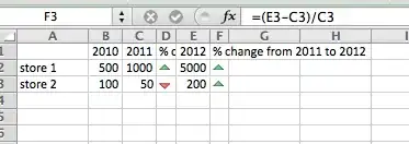
I have a table in Excel that looks something like this:

Stores        2010        2011        2012
---------------------------------------------
Store1       20000       30000       25000
Store2       60000       45000       50000
...
Store50      80000       41000       60000

I want to be able to create an icon set so that it will display an arrow pointing up, down or horizontal compared to its previous year. I've tried conditional formatting but it seems that it can't use relative cells.

So for example the above table would look something like:

Stores        2010        2011        2012
---------------------------------------------
Store1       20000      ^ 30000      v 25000
Store2       60000      v 45000      ^ 50000
...
Store50      80000      v 41000      ^ 60000

I found out that if i make a new conditional format for each cell I need it can be done, but with over 150 rows it would be nice to just create one format, and copy it to the other cells.

Can this be done?

Brian Tompsett - 汤莱恩
  • 5,753
  • 72
  • 57
  • 129
Caveman42
  • 679
  • 2
  • 13
  • 35

2 Answers2

1

I would suggest creating a new column and putting the % change from the previous to more recent year. Then do the conditional formatting on that row.

Is that an acceptable solution?

EDIT Screenshot below showing icon column can be narrowed to not show % change value.

enter image description here

Mark Silverberg
  • 1,249
  • 2
  • 8
  • 21
  • I could do that, but that would put the icons in a separate column, and I would like the icons to be next to the number. – Caveman42 Jul 29 '14 at 12:35
  • 1
    @Caveman42 understood. Added a screenshot to show that it is possible to make it not show the % change value – Mark Silverberg Jul 29 '14 at 12:38
  • Yea That is what I want, but I want the arrows to be in the same column as the number because I am using a pivot table, so I can't insert columns in the middle of it. I guess I could make a 2nd sheet and do a VLookUp? hmm.. – Caveman42 Jul 29 '14 at 12:40
  • My only other idea would be to use this 'hack' from http://stackoverflow.com/a/21420241/252671 to somehow embed the icon image into the cell using Google Docs and then export to Excel. Wouldn't suggest it but it might just work – Mark Silverberg Jul 29 '14 at 12:44
0

If the problem is with adding columns into a PT this could be overcome by adding calculated items for the changes, provided the data is 'flattened' first, but may involve a lot of formatting also:

SO25015298 example

The calculated items are of formula type:

='2011'/'2010'-1  

to return positive, negative or zero values that can then be formatted:

[Green]"ñ";[Red]"ò";[Yellow]"ó"  

with Bold Windings font.

The results appear unstable and may need to be reapplied on PT refresh.

pnuts
  • 58,317
  • 11
  • 87
  • 139