4

I have a little issue with calculating coordinates. Given are airfoil profiles in two lists with the following exemplary coordinates:

Example:

x_Coordinates = [1,   0.9,   0.7,   0.5,   0.3,   0.1, 0.0, ...] 
y_Coordinates = [0, -0.02, -0.06, -0.08, -0.10, -0.05, 0.0, ...]
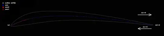
diagram 1: enter image description here

The only known things about the profile are the lists above and the following facts:

  • the first coordinate is always the trailing edge, in the example above at (x=1, y=0)
  • the coordinates always run on the bottom/underside to the leading edge, in the example above at (0,0) and from there back to the trailing edge
  • the profile is not normalized and it can exist in a rotated form

Now I want to determine

  1. the leading edge and
  2. the camber line.

Until now, I have always used the smallest x-coodinate as the leading edge. However, this would not work in the following exemplary profile, since the smallest x-coordinate is located on the upper surface of the profile.

diagram 2: enter image description here

Does anybody have an idea, how I could easily calculate/determine this data?


edit

one full sample array data

(1.0, 0.95, 0.9, 0.8, 0.7, 0.6, 0.5, 0.4, 0.3, 0.25, 0.2, 0.15, 0.1, 0.075, 0.05, 0.025, 0.0125, 0.005, 0.0, 0.005, 0.0125, 0.025, 0.05, 0.075, 0.1, 0.15, 0.2, 0.25, 0.3, 0.4, 0.5, 0.6, 0.7, 0.8, 0.9, 0.95, 1.0)
(0.00095, 0.00605, 0.01086, 0.01967, 0.02748, 0.03423, 0.03971, 0.04352, 0.04501, 0.04456, 0.04303, 0.04009, 0.03512, 0.0315, 0.02666, 0.01961, 0.0142, 0.0089, 0.0, -0.0089, -0.0142, -0.01961, -0.02666, -0.0315, -0.03512, -0.04009, -0.04303, -0.04456, -0.04501, -0.04352, -0.03971, -0.03423, -0.02748, -0.01967, -0.01086, -0.00605, -0.00095)
Spektre
  • 49,595
  • 11
  • 110
  • 380
René
  • 194
  • 1
  • 8
  • 1
    Its a bit tricky to compute the camber line if there's no corresponding point on the underside of the airfoil. What is the source of your data? Can you assume the leading edge is where the second derivate is biggest? – joojaa Sep 21 '14 at 14:17
  • Aso is it possible to get a full sample array data? – joojaa Sep 21 '14 at 14:26
  • Is it true that at the point of the leading edge, the [curvature is greatest](http://airfoiltools.com/airfoil/naca4digit)? – dbc Sep 21 '14 at 16:37
  • @joojaa thx for help. I added some sample data to my post. The source of my data are [cpacs files](https://code.google.com/p/cpacs/). These files will be created by several tools. – René Sep 21 '14 at 17:16
  • Looks like the profile data are actually stored in [Bernstein polynomial splines](ftp://ftp.heanet.ie/mirrors/sourceforge/c/cp/cpacs/CPACS_22_Schema.xsd). Could you use the [TiGL library](https://code.google.com/p/tigl/) to access and evaluate these curves? – dbc Sep 21 '14 at 19:25
  • @dbc I used [tixi library]https://code.google.com/p/tixi/ to access the data of the profiles but there are no other functions for evaluation. Thanks for the tigl hint , I 'll try it . – René Sep 21 '14 at 20:07
  • you should also post the nontrivial profile (on the bottom image) you provided the `symetric` sample data only ... – Spektre Sep 22 '14 at 09:38
  • You should reference this post [link](http://stackoverflow.com/questions/3783207/determining-a-mean-camber-line) – fang Sep 22 '14 at 17:11

2 Answers2

5

Well it was quite a few years I do something with wings.

I do not have any skewed wings data as on your image the closest thing I found was this:

wing

  1. leading edge not correct for nontrivial wings

    just find point where the sign of dx is flipping and compute

    dx(i)=x(i)-x(i-1)
    

    then mark zones where dx is positive or negative and find the middle between them (usually dx==0 for that zone). Mark the edge point as ix1

  2. camber line

    for precise geometry you will need intersections of normals casted from each side so:

    • start on outline point i
    • cast normal inside wing
    • search opposite side.
    • find point, It's normal intersect the opposite normal and divide both normals to the same distance

    This is doable but with insane complexity

  3. approximate camber line

    less precise way but much much faster so:

    1. start on outline point i
    2. find closest point to it on the opposite side
    3. compute midpoint between them and store it as inaccurate axis0 points. Do this for all points i=(0-ix1) (Red line)
    4. do the same but start from opposite side store as axis1 (dark red)
    5. when done then just find the average between axis0,axis1

    This can be done in the same way result is blue axis polyline

C++ source:

    List<double> pnt;   // outline 2D pnts = {x0,y0,x1,y1,x2,y2,...}
    List<double> axis;  // axis line 2D pnts = {x0,y0,x1,y1,x2,y2,...}
    int ix0,ix1;        // edge points

void compute()
    {
    int i,i0,i1;
    double d,dd;
    double *p0,*p1,*p2;
    double x0,x1,y0,y1;
    List<double> axis0,axis1;

    // find leading edge point
    ix0=0; ix1=0;
    for (p0=pnt.dat,p1=p0+2,p2=p1+2,i=2;i<pnt.num;i+=2,p0=p1,p1=p2,p2+=2)
     if ((p1[0]-p0[0])*(p2[0]-p1[0])<=0.0) { ix1=i; break; }
    // find axis0: midpoint of i0=(0-ix1) i1=find closest from (ix1,pnt.num)
    for (i0=2,i1=pnt.num-2;i0<ix1-2;i0+=2)
        {
        x0=pnt[i0+0];
        y0=pnt[i0+1];
        for (d=-1.0,i=i1;i>ix1+2;i-=2)
            {
            x1=pnt[i+0];
            y1=pnt[i+1];
            dd=((x1-x0)*(x1-x0))+((y1-y0)*(y1-y0));
            if ((d<0.0)||(dd<=d)) { i1=i; d=dd; }
            }
        if (d>=0.0)
            {
            x1=pnt[i1+0];
            y1=pnt[i1+1];
            axis0.add(0.5*(x0+x1));
            axis0.add(0.5*(y0+y1));
            }
        }
    // find axis1: midpoint of i0=(ix1,pnt.num) i1=find closest from (0,ix1)
    for (i1=2,i0=pnt.num-2;i0>ix1+2;i0-=2)
        {
        x0=pnt[i0+0];
        y0=pnt[i0+1];
        for (d=-1.0,i=i1;i<ix1-2;i+=2)
            {
            x1=pnt[i+0];
            y1=pnt[i+1];
            dd=((x1-x0)*(x1-x0))+((y1-y0)*(y1-y0));
            if ((d<0.0)||(dd<=d)) { i1=i; d=dd; }
            }
        if (d>=0.0)
            {
            x1=pnt[i1+0];
            y1=pnt[i1+1];
            axis1.add(0.5*(x0+x1));
            axis1.add(0.5*(y0+y1));
            }
        }
    // find axis: midpoint of i0=<0-axis0.num) i1=find closest from <0-axis1.num)
    axis.add(pnt[ix0+0]);
    axis.add(pnt[ix0+1]);
    for (i0=0,i1=0;i0<axis0.num;i0+=2)
        {
        x0=axis0[i0+0];
        y0=axis0[i0+1];
        for (d=-1.0,i=i1;i<axis1.num;i+=2)
            {
            x1=axis1[i+0];
            y1=axis1[i+1];
            dd=((x1-x0)*(x1-x0))+((y1-y0)*(y1-y0));
            if ((d<0.0)||(dd<=d)) { i1=i; d=dd; }
            }
        if (d>=0.0)
            {
            x1=axis1[i1+0];
            y1=axis1[i1+1];
            axis.add(0.5*(x0+x1));
            axis.add(0.5*(y0+y1));
            }
        }
    axis.add(pnt[ix1+0]);
    axis.add(pnt[ix1+1]);
    }
  • List<double> xxx; is just mine dynamic list template the same as double xxx[];
  • xxx.add(5); adds 5 to end of the list
  • xxx[7] access array element
  • xxx.num is the actual used size of the array
  • xxx.reset() clears the array and set xxx.num=0

[edit1] correct leading edge point

Have an insane thought about this to find the edge point on the run plus some code tweaking and the outcome is good enough for me :) so first some explaining:

enter image description here

algorithm for axis stays the same but instead of ix1 bound use only points that was not yet used ... Also count only valid closest points (on the opposite side) if none found stop (top image case). From this point find the most far point from last axis point this is the leading edge point.

This approach has much much accurate output (axis0,axis1 are closer together)

Now the C++ code:

void compute()
    {
    int i,i0,i1,ii,n=4;
    double d,dd;
    double x0,x1,y0,y1;
    List<double> axis0,axis1;
    ix0=0; ix1=0;

    // find axis0: midpoint of i0=(0-ix1) i1=find closest from (ix1,pnt.num)
    for (i0=0,i1=pnt.num-2;i0+n<i1;i0+=2)
        {
        x0=pnt[i0+0];
        y0=pnt[i0+1];
        i=i1+n; if (i>pnt.num-2) i=pnt.num-2; ii=i1;
        for (d=-1.0;i>i0+n;i-=2)
            {
            x1=pnt[i+0];
            y1=pnt[i+1];
            dd=((x1-x0)*(x1-x0))+((y1-y0)*(y1-y0));
            if ((d<0.0)||((dd<=d)&&(dd>1e-10))) { i1=i; d=dd; }
            if ((d>=0.0)&&(dd>d)) break;
            }
        if (d>=0.0)
            {
            if (i1-i0<=n+2) { i1=ii; break; } // stop if non valid closest point found
            x1=pnt[i1+0];
            y1=pnt[i1+1];
            axis0.add(0.5*(x0+x1));
            axis0.add(0.5*(y0+y1));
            }
        }
    // find leading edge point (the farest point from last found axis point)
    x0=axis0[axis0.num-2];
    y0=axis0[axis0.num-1];
    for (d=0.0,i=i0;i<=i1;i+=2)
        {
        x1=pnt[i+0];
        y1=pnt[i+1];
        dd=((x1-x0)*(x1-x0))+((y1-y0)*(y1-y0));
        if (dd>d) { ix1=i; d=dd; }
        }
    axis0.add(pnt[ix1+0]);
    axis0.add(pnt[ix1+1]);

    // find axis1: midpoint of i0=(ix1,pnt.num) i1=find closest from (0,ix1)
    for (i1=0,i0=pnt.num-2;i0+n>i1;i0-=2)
        {
        x0=pnt[i0+0];
        y0=pnt[i0+1];
        i=i1-n; if (i<0) i=0; ii=i1;
        for (d=-1.0;i<i0-n;i+=2)
            {
            x1=pnt[i+0];
            y1=pnt[i+1];
            dd=((x1-x0)*(x1-x0))+((y1-y0)*(y1-y0));
            if ((d<0.0)||((dd<=d)&&(dd>1e-10))) { i1=i; d=dd; }
            if ((d>=0.0)&&(dd>d)) break;
            }
        if (d>=0.0)
            {
            if (i0-i1<=n+2) { i1=ii; break; } // stop if non valid closest point found
            x1=pnt[i1+0];
            y1=pnt[i1+1];
            axis1.add(0.5*(x0+x1));
            axis1.add(0.5*(y0+y1));
            }
        }
    // find leading edge point (the farest point from last found axis point)
    x0=axis1[axis1.num-2];
    y0=axis1[axis1.num-1];
    for (d=0.0,i=i1;i<=i0;i+=2)
        {
        x1=pnt[i+0];
        y1=pnt[i+1];
        dd=((x1-x0)*(x1-x0))+((y1-y0)*(y1-y0));
        if (dd>d) { ix1=i; d=dd; }
        }
    axis1.add(pnt[ix1+0]);
    axis1.add(pnt[ix1+1]);

    // find axis: midpoint of i0=<0-axis0.num) i1=find closest from <0-axis1.num)
    for (i0=0,i1=0;i0<axis0.num;i0+=2)
        {
        x0=axis0[i0+0];
        y0=axis0[i0+1];
        for (d=-1.0,i=i1;i<axis1.num;i+=2)
            {
            x1=axis1[i+0];
            y1=axis1[i+1];
            dd=((x1-x0)*(x1-x0))+((y1-y0)*(y1-y0));
            if ((d<0.0)||(dd<=d)) { i1=i; d=dd; }
            }
        if (d>=0.0)
            {
            x1=axis1[i1+0];
            y1=axis1[i1+1];
            axis.add(0.5*(x0+x1));
            axis.add(0.5*(y0+y1));
            }
        }
    }

constant n=4 is just for safety overlapped search for closest points it should be a fraction of pnt.num. Sometimes the closest point is before the last found closest point this depends on the curvature of booth sides. Too big n will cause slowdowns and if n>pnt.num/4 it could also invalidate output.

If too small then for smaller radius of curvature will lower the accuracy this approach is dependent on sufficient point coverage. If the wing is sampled with too low point count it can lead to inaccuracy. The source code is 3 times almost the same thing you can chose which ix1 to remember (from first or second search) they are neighboring points

test profile:

1.000000 0.000000
0.990000 0.006719
0.980000 0.013307
0.970000 0.019757
0.960000 0.026064
0.950000 0.032223
0.940000 0.038228
0.930000 0.044075
0.920000 0.049759
0.910000 0.055276
0.900000 0.060623
0.890000 0.065795
0.880000 0.070790
0.870000 0.075604
0.860000 0.080234
0.850000 0.084678
0.840000 0.088935
0.830000 0.093001
0.820000 0.096876
0.810000 0.100558
0.800000 0.104046
0.790000 0.107339
0.780000 0.110438
0.770000 0.113342
0.760000 0.116051
0.750000 0.118566
0.740000 0.120887
0.730000 0.123016
0.720000 0.124954
0.710000 0.126702
0.700000 0.128262
0.690000 0.129637
0.680000 0.130829
0.670000 0.131839
0.660000 0.132672
0.650000 0.133331
0.640000 0.133818
0.630000 0.134137
0.620000 0.134292
0.610000 0.134287
0.600000 0.134127
0.590000 0.133815
0.580000 0.133356
0.570000 0.132755
0.560000 0.132016
0.550000 0.131146
0.540000 0.130148
0.530000 0.129030
0.520000 0.127795
0.510000 0.126450
0.500000 0.125000
0.490000 0.123452
0.480000 0.121811
0.470000 0.120083
0.460000 0.118275
0.450000 0.116392
0.440000 0.114441
0.430000 0.112429
0.420000 0.110361
0.410000 0.108244
0.400000 0.106085
0.390000 0.103889
0.380000 0.101663
0.370000 0.099414
0.360000 0.097148
0.350000 0.094870
0.340000 0.092589
0.330000 0.090309
0.320000 0.088037
0.310000 0.085779
0.300000 0.083541
0.290000 0.081329
0.280000 0.079149
0.270000 0.077006
0.260000 0.074906
0.250000 0.072855
0.240000 0.070858
0.230000 0.068920
0.220000 0.067047
0.210000 0.065242
0.113262 0.047023
0.110002 0.042718
0.106385 0.038580
0.102428 0.034615
0.098146 0.030832
0.093556 0.027239
0.088673 0.023844
0.083516 0.020652
0.078101 0.017670
0.072448 0.014904
0.066574 0.012361
0.060499 0.010044
0.054241 0.007958
0.047820 0.006108
0.041256 0.004497
0.034569 0.003129
0.027779 0.002005
0.020907 0.001129
0.013972 0.000502
0.006997 0.000126
0.000000 0.000000
0.000000 0.000000
-0.003997 0.000126
-0.007972 0.000502
-0.011907 0.001129
-0.015779 0.002005
-0.019569 0.003129
-0.023256 0.004497
-0.026820 0.006108
-0.030241 0.007958
-0.033499 0.010044
-0.036574 0.012361
-0.039448 0.014904
-0.042101 0.017670
-0.044516 0.020652
-0.046673 0.023844
-0.048556 0.027239
-0.050146 0.030832
-0.051428 0.034615
-0.052385 0.038580
-0.053002 0.042718
-0.053262 0.047023
-0.053153 0.051484
-0.052659 0.056093
-0.051768 0.060841
-0.050467 0.065717
-0.048744 0.070711
-0.046588 0.075813
-0.043988 0.081012
-0.040935 0.086297
-0.037420 0.091658
-0.033435 0.097082
-0.028972 0.102558
-0.024025 0.108074
-0.018589 0.113618
-0.012657 0.119178
-0.006228 0.124741
0.000704 0.130295
0.008139 0.135828
0.016079 0.141326
0.024525 0.146777
0.033475 0.152169
0.042930 0.157488
0.052885 0.162722
0.063339 0.167858
0.074287 0.172883
0.085723 0.177784
0.097643 0.182549
0.110038 0.187166
0.122902 0.191621
0.136226 0.195903
0.150000 0.200000
0.164214 0.203899
0.178856 0.207590
0.193914 0.211059
0.209376 0.214297
0.225227 0.217291
0.241453 0.220032
0.258039 0.222509
0.274968 0.224711
0.292223 0.226629
0.309787 0.228254
0.327641 0.229575
0.345766 0.230585
0.364142 0.231274
0.382749 0.231636
0.401566 0.231662
0.420570 0.231345
0.439740 0.230679
0.459054 0.229657
0.478486 0.228274
0.498015 0.226525
0.517615 0.224404
0.537262 0.221908
0.556930 0.219032
0.576595 0.215775
0.596231 0.212132
0.615811 0.208102
0.635310 0.203684
0.654700 0.198876
0.673956 0.193679
0.693050 0.188091
0.711955 0.182115
0.730644 0.175751
0.749091 0.169002
0.767268 0.161869
0.785149 0.154357
0.802706 0.146468
0.819913 0.138207
0.836742 0.129580
0.853169 0.120591
0.869166 0.111246
0.884707 0.101553
0.899768 0.091518
0.914322 0.081149
0.928345 0.070455
0.941813 0.059445
0.954701 0.048128
0.966987 0.036514
0.978646 0.024614
0.989658 0.012439
1.000000 0.000000
Spektre
  • 49,595
  • 11
  • 110
  • 380
  • thx for your solution. Your idea with the approximate camber line is great. I currently develop a tool which reads profile data out of cpacs files. These profiles can be unconventionally or can be stored in a rotated way. My central issue is to compute the leading edge for such profiles. I found the nontrivial wing on [wikipedia](http://en.wikipedia.org/wiki/Chord_%28aeronautics%29). Therefore I have currently no data of this profile. – René Sep 22 '14 at 13:58
  • @René I am currently looking at the leading edge point for nontrivial wing (I found only image no dat file for that profile it is turbine blade not wing) had ported mine old wing class code to newer compiler for this I approximate the airfoil with some sin,cos functions and now I inspecting one interesting way to find the edge point during the axis search itself. Funny how 10+ years code looks like in comparison to nowadays code style of mine :) – Spektre Sep 22 '14 at 14:13
  • @René I did it ... added edit1 to my answer. I know it is a bit sketchy but it works also added mine approximated profile – Spektre Sep 22 '14 at 15:37
  • wow thats cool, it may seem to work well at first :-) Thanks a lot. – René Sep 22 '14 at 16:43
  • @René it works well for almost all of mine profiles. I found only one that is not OK (one search is OK and the second not) but that is almost certainly a bug in profile file because very similar profiles to it works OK (mine old profiles are very buggy from old automated measuring system for planes) the data is jittery and need some smoothing (that is what the original code of mine was for btw it was mine first commercial product :) ) ... glad to be of help... – Spektre Sep 22 '14 at 16:49
-1

A little outdated, but I still came across this post.

My solution for the leading edge circle is to first interpolate a spline through the airfoil coordinates. This gives a smooth parametric representation of the airfoil. Then calculate the curvature and curvature circles for the parametric curve and take the smallest circle. This defines the leading edge position and returns the radius there as well.

Below there are two Python functions (relying on the numpy and scipy packages) doing that:

def spline(self, x, y, points=200, degree=2, evaluate=False):
    """Interpolate spline through given points

    Args:
        spline (int, optional): Number of points on the spline
        degree (int, optional): Degree of the spline
        evaluate (bool, optional): If True, evaluate spline just at
                                   the coordinates of the knots
    """

    # interpolate B-spline through data points
    # returns knots of control polygon
    # tck ... tuple (t,c,k) containing the vector of knots,
    # the B-spline coefficients, and the degree of the spline.
    # u ... array of the parameters for each knot
    # NOTE: s=0.0 is important as no smoothing should be done on the spline
    # after interpolating it
    tck, u = interpolate.splprep([x, y], s=0.0, k=degree)

    # number of points on interpolated B-spline (parameter t)
    t = np.linspace(0.0, 1.0, points)

    # if True, evaluate spline just at the coordinates of the knots
    if evaluate:
        t = u

    # evaluate B-spline at given parameters
    # der=0: returns point coordinates
    coo = interpolate.splev(t, tck, der=0)

    # evaluate 1st derivative at given parameters
    der1 = interpolate.splev(t, tck, der=1)

    # evaluate 2nd derivative at given parameters
    der2 = interpolate.splev(t, tck, der=2)

    spline_data = [coo, u, t, der1, der2, tck]

    return spline_data

Function to calculate the curvature properties of a parametric curve:

    def getCurvature(spline_data):
    """Curvature and radius of curvature of a parametric curve

    der1 is dx/dt and dy/dt at each point
    der2 is d2x/dt2 and d2y/dt2 at each point

    Returns:
        float: Tuple of numpy arrays carrying gradient of the curve,
               the curvature, radiusses of curvature circles and
               curvature circle centers for each point of the curve
    """

    coo = spline_data[0]
    der1 = spline_data[3]
    der2 = spline_data[4]

    xd = der1[0]
    yd = der1[1]
    x2d = der2[0]
    y2d = der2[1]
    n = xd**2 + yd**2
    d = xd*y2d - yd*x2d

    # gradient dy/dx = dy/du / dx/du
    gradient = der1[1] / der1[0]

    # radius of curvature
    R = n**(3./2.) / abs(d)

    # curvature
    C = d / n**(3./2.)

    # coordinates of curvature-circle center points
    xc = coo[0] - R * yd / np.sqrt(n)
    yc = coo[1] + R * xd / np.sqrt(n)

    return [gradient, C, R, xc, yc]

Example: enter image description here

Detail: enter image description here

Note that I also use a refinement of the spline at the leading edge. The corresponding algorithm is not presented here (as off topic).

chiefenne
  • 565
  • 2
  • 15
  • 30