how to snip or crop or white-fill a large. expanded (by 10%) rectangle outside of a polygon with ggplot2

Question

this question is a follow-up of my prior SO question and is related to this question.

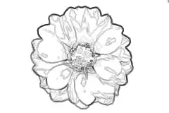
i'm just trying to white-fill an area 10% bigger than a simple polygon with ggplot2. maybe i'm grouping things wrong? here's a photo of the spike with reproducible code below

# reproducible example
library(rgeos)
library(maptools)
library(raster)

shpct.tf <- tempfile() ; td <- tempdir()

download.file( 
    "ftp://ftp2.census.gov/geo/pvs/tiger2010st/09_Connecticut/09/tl_2010_09_state10.zip" ,
    shpct.tf ,
    mode = 'wb'
)

shpct.uz <- unzip( shpct.tf , exdir = td )

# read in connecticut
ct.shp <- readShapePoly( shpct.uz[ grep( 'shp$' , shpct.uz ) ] )

# box outside of connecticut
ct.shp.env <- gEnvelope( ct.shp )
ct.shp.out <- as( 1.2 * extent( ct.shp ), "SpatialPolygons" )


# difference between connecticut and its box
ct.shp.env.diff <- gDifference( ct.shp.env , ct.shp )
ct.shp.out.diff <- gDifference( ct.shp.out , ct.shp )


library(ggplot2)


# prepare both shapes for ggplot2
f.ct.shp <- fortify( ct.shp )
env <- fortify( ct.shp.env.diff )
outside <- fortify( ct.shp.out.diff )


# create all layers + projections
plot <- ggplot(data = f.ct.shp, aes(x = long, y = lat))  #start with the base-plot 

layer1 <- geom_polygon(data=f.ct.shp, aes(x=long,y=lat), fill='black')

layer2 <- geom_polygon(data=env, aes(x=long,y=lat,group=group), fill='white')

layer3 <- geom_polygon(data=outside, aes(x=long,y=lat,group=id), fill='white')

co <- coord_map( project = "albers" , lat0 = 40.9836 , lat1 = 42.05014 )

# this works
plot + layer1 

# this works
plot + layer2

# this works
plot + layer1 + layer2

# this works
plot + layer2 + co

# this works
plot + layer1 + layer3

# here's the problem: this breaks
plot + layer3 + co

# this also breaks, but it's ultimately how i want to display things
plot + layer1 + layer3 + co

# this looks okay in this example but
# does not work for what i'm trying to do-
# cover up points outside of the state
plot + layer3 + layer1 + co

Answer 1

This is because `coord_map', or more generally non-linear coordinates, internally interpolates vertices so that line is draw as a curve corresponding the coordinate. In your case, interpolation will be performed between a point of the outer rectangle and a point of inner edge, which you see as the break.

You can change this by:

co2 <- co
class(co2) <- c("hoge", class(co2))
is.linear.hoge <- function(coord) TRUE
plot + layer1 + layer3 + co2

You can also find the difference of behavior here:

ggplot(data.frame(x = c(0, 90), y = 45), aes(x, y)) + geom_line() + co + ylim(0, 90)

ggplot(data.frame(x = c(0, 90), y = 45), aes(x, y)) + geom_line() + co2 + ylim(0, 90)

Answer 2

Here's how I'd go about it with base plotting functions. It wasn't entirely clear to me whether you need the "background" polygon to be differences against the state polygon, or whether it's fine for it to be a simple rectangle that will have the state poly overlain. Either is possible, but I'll do the latter here for brevity/simplicity.

library(rgdal)
library(raster) # for extent() and crs() convenience

# download, unzip, and read in shapefile
download.file(file.path('ftp://ftp2.census.gov/geo/pvs/tiger2010st/09_Connecticut/09',
                        'tl_2010_09_state10.zip'), f <- tempfile(), mode='wb')
unzip(f, exdir=tempdir())
ct <- readOGR(tempdir(), 'tl_2010_09_state10')

# define albers and project ct
# I've set the standard parallels inwards from the latitudinal limits by one sixth of
# the latitudinal range, and the central meridian to the mid-longitude. Lat of origin 
# is arbitrary since we transform it back to longlat anyway.
alb <- CRS('+proj=aea +lat_1=41.13422 +lat_2=41.86731 +lat_0=0 +lon_0=-72.75751
           +x_0=0 +y_0=0 +ellps=GRS80 +towgs84=0,0,0,0,0,0,0 +units=m +no_defs')
ct.albers <- spTransform(ct, alb)

# expand bbox by 10% and make a polygon of this extent
buf <- as(1.2 * extent(ct.albers), 'SpatialPolygons')
proj4string(buf) <- alb

# plot without axes
par(mar=c(6, 5, 1, 1)) # space for axis labels
plot(buf, col='white', border=NA)
do.call(rect, as.list(c(par('usr')[c(1, 3, 2, 4)], col='gray90'))) 
# the above line is just in case you needed the grey bg
plot(buf, add=TRUE, col='white', border=NA) # add the buffer
plot(ct.albers, add=TRUE, col='gray90', border=NA)
title(xlab='Longitude')
title(ylab='Latitude', line=4)

Now, if I understand correctly, despite being in a projected coordinate system, you want to plot axes that are in the units of another (the original) coordinate system. Here's a function that can do that for you.

[EDIT: I've made some changes to the following code. It now (optionally) plots the grid lines, which are particularly important when plotting axis in units that are in a different projection to the plot.]

axis.crs <- function(plotCRS, axisCRS, grid=TRUE, lty=1, col='gray', ...) {
  require(sp)
  require(raster)
  e <- as(extent(par('usr')), 'SpatialPolygons')
  proj4string(e) <- plotCRS
  e.ax <- spTransform(e, axisCRS)
  if(isTRUE(grid)) lines(spTransform(gridlines(e.ax), plotCRS), lty=lty, col=col)
  axis(1, coordinates(spTransform(gridat(e.ax), plotCRS))[gridat(e.ax)$pos==1, 1],
       parse(text=gridat(e.ax)$labels[gridat(e.ax)$pos==1]), ...)
  axis(2, coordinates(spTransform(gridat(e.ax), plotCRS))[gridat(e.ax)$pos==2, 2],
       parse(text=gridat(e.ax)$labels[gridat(e.ax)$pos==2]), las=1, ...)
  box(lend=2) # to deal with cases where axes have been plotted over the original box
}

axis.crs(alb, crs(ct), cex.axis=0.8, lty=3)