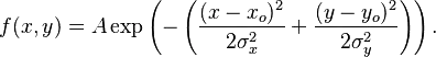
That's pretty easy to achieve with meshgrid. You'll need to generate a set of X and Y points, then use these as input into two Gaussian functions with known means and standard deviations. Once you do this, you just have to sum them together, then you can visualize this using mesh. Recall the definition of a 2D Gaussian:
Source: Wikipedia
Small Note: Referencing the comments of this post, Amro made a good observation where we are assuming that the covariance matrix of the given distribution is diagonal. This means that each dimension of your data do not co-vary with each other and are independent. Should this not be the case, then this will require a bit more complicated computations, but can easily be achievable using matrix operations: https://en.wikipedia.org/wiki/Multivariate_normal_distribution#Density_function. Since you haven't really given me any information about the distribution of your data, I'm going to assume that each dimension doesn't co-vary, and you have a diagonal covariance matrix. You can also check out his post here if you want to see a more detailed and more general case on how to plot a mixture of 2D Gaussians: https://stackoverflow.com/a/26070081/97160
x_0 and y_0 are the mean in the x and y direction while o_x and o_y denote the standard deviation in the x and y directions. A is a normalizing constant, which is usually 1 for simplicity. You just need to generate a grid of co-ordinates that span between some known dimensions, then specify 2 pairs of means and standard deviations, run through this expression for each of these parameters then show the result after adding the two. Let's assume that the grid spans between -10 <= (x,y) <= 10. Also, let's say our means and standard deviations were the following for this example:
x_1 = 2
x_2 = 2
y_1 = -1
y_2 = -1

o_x_1 = 1
o_y_1 = 2
o_x_2 = 2
o_y_2 = 1
As such, x_1, y_1 are the means for the x and y directions of the first Gaussian, x_2, y_2 are the means for the second Gaussian, o_x_1, o_y_1 are the standard deviations of the first Gaussian in the x and y directions and o_x_2, o_y_2 are the standard deviations of the second Gaussian in the x and y directions. Therefore, your code really just needs to do this:
%// Define grid of points
[X,Y] = meshgrid(-10:0.01:10, -10:0.01:10);

%// Define parameters for each Gaussian
x_1 = 2;
y_1 = 2;
x_2 = -1;
y_2 = -1;

o_x_1 = 1;
o_y_1 = 2;
o_x_2 = 2;
o_y_2 = 1;

%// Define constant A... let's just assume 1 for both
A = 1;

%// Generate Gaussian values for both Gaussians
f1 = A*exp( -( ((X - x_1).^2 / (2*o_x_1^2)) + ((Y - y_1).^2 / (2*o_y_1^2)) ) );
f2 = A*exp( -( ((X - x_2).^2 / (2*o_x_2^2)) + ((Y - y_2).^2 / (2*o_y_2^2)) ) );

%// Add them up
f = f1 + f2;

%// Show the results
mesh(X, Y, f);
%// Label the axes
xlabel('x');
ylabel('y');
zlabel('z');
view(-130,50); %// For a better view
colorbar; %// Add a colour bar for good measure
Here's the plot I get, once I adjust the viewing camera for a better viewing angle, as well as showing a colour bar on the right of the figure to illustrate a visual representation of the heights for the plot.
To appreciate how these two are mixing, let's point the camera directly above. You can adjust the viewing angle to move the camera directly above the plot by:
view(0, 90);
This is what I get:

With the above figure, it's more obvious as to what we are doing. You can see where the Gaussians are centered at. Specifically, (x,y) = (2,2) for the first Gaussian and (x,y) = (-1,-1) for the second Gaussian.
You also get to see them merge as there are tails on each of the Gaussians that eventually touch each other, and when you add them up you see this merging effect. Also, the general shape of the Gaussians are what we expect. For the first one centered at (x,y) = (2,2), I made the horizontal standard deviation 1 while the vertical standard deviation 2, so it would naturally be taller with respect to the y direction. Similarly, for the second one centered at (x,y) = (-1,-1), I flipped the standard deviations, so we would expect this to be wider with respect to the x direction.
This is something you can start with. I really don't know what your end application is, but perhaps this code can help you along the way. I did my best given your problem description.
Have fun!