This question is similar to Fit a non-linear function to data/observations with pyMCMC/pyMC, in that I'm trying to do nonlinear regression using PyMC.
However, I was wondering if anyone knew how to make my observed variable follow a non-normal distribution (i.e., T distribution) using PyMC. I know they include T distributions, but I wasn't sure how to include these as my observed variable.
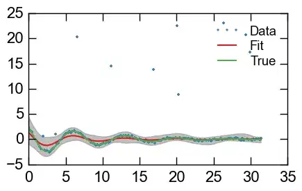
Here's a quick demonstration using some faked-up data of where I'm running into issues: I'd like to use an output distribution that protects against some of the clearly outlier data points.
import numpy as np
import pymc as pm
import matplotlib.pyplot as plt

# For reproducibility
np.random.seed(1234)

x = np.linspace(0, 10*np.pi, num=150)

# Set real parameters for the sinusoid
true_freq = 0.9
true_logamp = 1.2
true_decay = 0.12
true_phase = np.pi/4


# Simulate the true trajectory
y_real = (np.exp(true_logamp - true_decay*x) *
          np.cos(true_freq*x + true_phase))

# Add some noise
y_err = y_real + 0.05*y_real.max()*np.random.randn(len(x))


# Add some outliers
num_outliers = 10
outlier_locs = np.random.randint(0, len(x), num_outliers)
y_err[outlier_locs] += (10 * y_real.max() *
                        (np.random.rand(num_outliers)))


# Bayesian Regression

def model(x, y, p0):

    log_amp = pm.Normal('log_amp', mu=np.log(p0['amplitude']),
                        tau=1/(np.log(p0['amplitude'])))

    decay = pm.Normal('decay', mu=p0['decay'],
                        tau=1/(p0['decay']))

    period = pm.TruncatedNormal('period', mu=p0['period'],
                                tau=1/(p0['period']),
                                a=1/(0.5/(np.median(np.diff(x)))),
                                b=x.max() - x.min())

    phase = pm.VonMises('phase', mu=p0['phase'], kappa=1.)

    obs_tau = pm.Gamma('obs_tau', 0.1, 0.1)

    @pm.deterministic(plot=False)
    def decaying_sinusoid(x=x, log_amp=log_amp, decay=decay,
                          period=period, phase=phase):

        return (np.exp(log_amp - decay*x) *
                np.cos((2*np.pi/period)*x + phase))

    obs = pm.Normal('obs', mu=decaying_sinusoid, tau=obs_tau, value=y,
                    observed=True)

    return locals()

p0 = {
    'amplitude' : 2.30185,
    'decay'     : 0.06697,
    'period'    : 7.11672,
    'phase'     : 0.93055,
}


MDL = pm.MCMC(model(x, y_err, p0))
MDL.sample(20000, 10000, 1)

# Plot fit
y_min = MDL.stats()['decaying_sinusoid']['quantiles'][2.5]
y_max = MDL.stats()['decaying_sinusoid']['quantiles'][97.5]
y_fit = MDL.stats()['decaying_sinusoid']['mean']
plt.plot(x, y_err, '.', label='Data')
plt.plot(x, y_fit, label='Fit')
plt.plot(x, y_real, label='True')

plt.fill_between(x, y_min, y_max, color='0.5', alpha=0.5)
plt.legend()
Thanks!!