Curve fitting: Find the smoothest function that satisfies a list of constraints

Question

Consider the set of non-decreasing surjective (onto) functions from (-inf,inf) to [0,1]. (Typical CDFs satisfy this property.) In other words, for any real number x, 0 <= f(x) <= 1. The logistic function is perhaps the most well-known example.

We are now given some constraints in the form of a list of x-values and for each x-value, a pair of y-values that the function must lie between. We can represent that as a list of {x,ymin,ymax} triples such as

constraints = {{0, 0, 0}, {1, 0.00311936, 0.00416369}, {2, 0.0847077, 0.109064}, 
 {3, 0.272142, 0.354692}, {4, 0.53198, 0.646113}, {5, 0.623413, 0.743102}, 
 {6, 0.744714, 0.905966}}

Graphically that looks like this:

_{(source: yootles.com)}

We now seek a curve that respects those constraints. For example:

_{(source: yootles.com)}

Let's first try a simple interpolation through the midpoints of the constraints:

mids = ({#1, Mean[{#2,#3}]}&) @@@ constraints
f = Interpolation[mids, InterpolationOrder->0]

Plotted, f looks like this:

_{(source: yootles.com)}

That function is not surjective. Also, we'd like it to be smoother. We can increase the interpolation order but now it violates the constraint that its range is [0,1]:

_{(source: yootles.com)}

The goal, then, is to find the smoothest function that satisfies the constraints:

1. Non-decreasing.
2. Tends to 0 as x approaches negative infinity and tends to 1 as x approaches infinity.
3. Passes through a given list of y-error-bars.

The first example I plotted above seems to be a good candidate but I did that with Mathematica's FindFit function assuming a lognormal CDF. That works well in this specific example but in general there need not be a lognormal CDF that satisfies the constraints.

Answer 1

I don't think you've specified enough criteria to make the desired CDF unique.

If the only criteria that must hold is:

1. CDF must be "fairly smooth" (see below)
2. CDF must be non-decreasing
3. CDF must pass through the "error bar" y-intervals
4. CDF must tend toward 0 as x --> -Infinity
5. CDF must tend toward 1 as x --> Infinity.

then perhaps you could use Monotone Cubic Interpolation. This will give you a C^2 (twice continously differentiable) function which, unlike cubic splines, is guaranteed to be monotone when given monotone data.

This leaves open the question, exactly what data should you use to generate the monotone cubic interpolation. If you take the center point (mean) of each error bar, are you guaranteed that the resulting data points are monotonically increasing? If not, you might as well make some arbitrary choice to guarantee that the points you select are monotonically increasing (because the criteria does not force our solution to be unique).

Now what to do about the last data point? Is there an X which is guaranteed to be larger than any x in the constraints data set? Perhaps you can again make an arbitrary choice of convenience and pick some very large X and put (X,1) as the final data point.

Comment 1: Your problem can be broken into 2 sub-problems:

1. Given exact points (x_i,y_i) through which the CDF must pass, how do you generate CDF? I suspect there are infinitely many possible solutions, even with the infinite-smoothness constraint.

2. Given y-errorbars, how should you pick (x_i,y_i)? Again, there infinitely many possible solutions. Some additional criteria may need to be added to force a unique choice. Additional criteria would also probably make the problem even harder than it currently is.

Comment 2: Here is a way to use monotonic cubic interpolation, and satisfy criteria 4 and 5:

The monotonic cubic interpolation (let's call it f) maps R --> R.

Let CDF(x) = exp(-exp(f(x))). Then CDF: R --> (0,1). If we could find the appropriate f, then by defining CDF this way, we could satisfy criteria 4 and 5.

To find f, transform the CDF constraints (x_0,y_0),...,(x_n,y_n) using the transformation xhat_i = x_i, yhat_i = log(-log(y_i)). This is the inverse of the CDF transformation. If the y_i's were increasing, then the yhat_i's are decreasing.

Now apply monotone cubic interpolation to the (x_hat,y_hat) data points to generate f. Then finally, define CDF(x) = exp(-exp(f(x))). This will be a monotonically increasing function from R --> (0,1), which passes through the points (x_i,y_i).

This, I think, satisfies all the criteria 2--5. Criteria 1 is somewhat satisfied, though there certainly could exist smoother solutions.

Answer 2

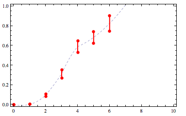
I have found a solution that gives reasonable results for a variety of inputs. I start by fitting a model -- once to the low ends of the constraints, and again to the high ends. I'll refer to the mean of these two fitted functions as the "ideal function". I use this ideal function to extrapolate to the left and to the right of where the constraints end, as well as to interpolate between any gaps in the constraints. 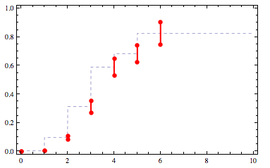I compute values for the ideal function at regular intervals, including all the constraints, from where the function is nearly zero on the left to where it's nearly one on the right. At the constraints, I clip these values as necessary to satisfy the constraints. Finally, I construct an interpolating function that goes through these values.

My Mathematica implementation follows.
First, a couple helper functions:

(* Distance from x to the nearest member of list l. *)
listdist[x_, l_List] := Min[Abs[x - #] & /@ l]

(* Return a value x for the variable var such that expr/.var->x is at least (or
   at most, if dir is -1) t. *)
invertish[expr_, var_, t_, dir_:1] := Module[{x = dir},
  While[dir*(expr /. var -> x) < dir*t, x *= 2];
  x]

And here's the main function:

(* Return a non-decreasing interpolating function that maps from the
   reals to [0,1] and that is as close as possible to expr[var] without
   violating the given constraints (a list of {x,ymin,ymax} triples).
   The model, expr, will have free parameters, params, so first do a
   model fit to choose the parameters to satisfy the constraints as well
   as possible. *)
cfit[constraints_, expr_, params_, var_] := 
Block[{xlist,bots,tops,loparams,hiparams,lofit,hifit,xmin,xmax,gap,aug,bests},
  xlist = First /@ constraints;
  bots = Most /@ constraints; (* bottom points of the constraints *)
  tops = constraints /. {x_, _, ymax_} -> {x, ymax};
  (* fit a model to the lower bounds of the constraints, and 
     to the upper bounds *)
  loparams = FindFit[bots, expr, params, var];
  hiparams = FindFit[tops, expr, params, var];
  lofit[z_] = (expr /. loparams /. var -> z);
  hifit[z_] = (expr /. hiparams /. var -> z);
  (* find x-values where the fitted function is very close to 0 and to 1 *)
  {xmin, xmax} = {
    Min@Append[xlist, invertish[expr /. hiparams, var, 10^-6, -1]],
    Max@Append[xlist, invertish[expr /. loparams, var, 1-10^-6]]};
  (* the smallest gap between x-values in constraints *)
  gap = Min[(#2 - #1 &) @@@ Partition[Sort[xlist], 2, 1]];
  (* augment the constraints to fill in any gaps and extrapolate so there are 
     constraints everywhere from where the function is almost 0 to where it's 
     almost 1 *)
  aug = SortBy[Join[constraints, Select[Table[{x, lofit[x], hifit[x]}, 
                                              {x, xmin,xmax, gap}], 
                                        listdist[#[[1]],xlist]>gap&]], First];
  (* pick a y-value from each constraint that is as close as possible to 
     the mean of lofit and hifit *)
  bests = ({#1, Clip[(lofit[#1] + hifit[#1])/2, {#2, #3}]} &) @@@ aug;
  Interpolation[bests, InterpolationOrder -> 3]]

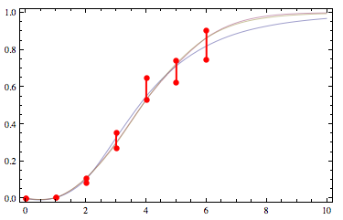
For example, we can fit to a lognormal, normal, or logistic function:

g1 = cfit[constraints, CDF[LogNormalDistribution[mu,sigma], z], {mu,sigma}, z]
g2 = cfit[constraints, CDF[NormalDistribution[mu,sigma], z], {mu,sigma}, z]
g3 = cfit[constraints, 1/(1 + c*Exp[-k*z]), {c,k}, z]

Here's what those look like for my original list of example constraints:

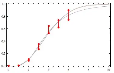
_{(source: yootles.com)}

The normal and logistic are nearly on top of each other and the lognormal is the blue curve.

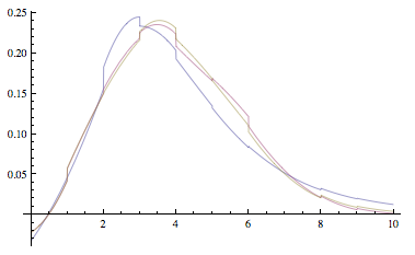
These are not quite perfect. In particular, they aren't quite monotone. Here's a plot of the derivatives:

Plot[{g1'[x], g2'[x], g3'[x]}, {x, 0, 10}]

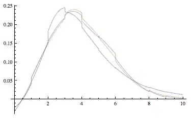
_{(source: yootles.com)}

That reveals some lack of smoothness as well as the slight non-monotonicity near zero. I welcome improvements on this solution!

Answer 3

You can try to fit a Bezier curve through the midpoints. Specifically I think you want a C2 continuous curve.