Related to: Cross Stitch to Matlab
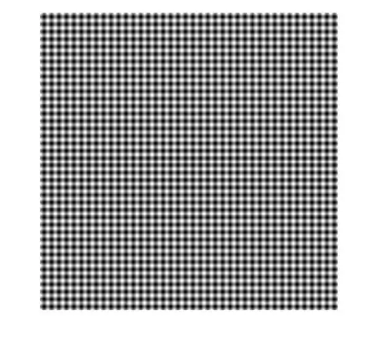
How can I create a cross Stitch pattern over a pixelated image?
Something like:
where each pixel has a X like pattern on top of it.
Related to: Cross Stitch to Matlab
How can I create a cross Stitch pattern over a pixelated image?
Something like:
where each pixel has a X like pattern on top of it.
Here's my one attempt to try and create cross-stitched images in MATLAB. One technique that I have seen is to take the Fourier Transform of your image and strategically replace locations in the spectrum with very large magnitudes. The intuition behind this can be shown by an awesome image processing slide by Richard Alan Peters II from his Frequency Domain discussion. I'm attaching the picture below, you can refer to the original slides here on page 50.
Essentially, if you place a single point (or it should be pairs actually as this is the complex plane and so we should have conjugate pairs) on the spectrum, it defines a spatial frequency as well as an angle that the intensities oscillate at. Bear in mind that this is for a spectrum where there is only one point. If you want to mimic a cross stitch pattern, you'll want to place four points around the DC component (centre). You'll want to place them in the north, south, east and west directions. The intuition behind this is that by placing two points horizontally with respect to the centre, we would get spatial oscillations that oscillate from left to right. Similarly, if we place two points vertically with respect to the centre, we get oscillations from top to bottom. By combining these two, we would simulate a checkerboard pattern.
Here's an example where I've created a 512 x 512 image, and have placed high magnitudes in such a grid that is 20 pixels away from the centre:
A = zeros(512, 512);
r = 20;
rows_half = floor(size(A,1)/2) + 1;
cols_half = floor(size(A,2)/2) + 1;
A(rows_half-r,cols_half) = 1000;
A(rows_half,cols_half-r) = 1000;
A(rows_half+r,cols_half) = 1000;
A(rows_half,cols_half+r) = 1000;
Ashift = ifftshift(A);
out = real(ifft2(Ashift));
imshow(out, []);
This is what I get for the image:
Cool huh? Now, you probably want to make the spacing between the squares "tighter", and that means you need to make the frequency larger. As such, you simply just need to change how far each point is with respect to the centre, so maybe increase this to 40? Set r to 40, and we get:
.... r = 80?

Much better! The point with this demonstration is that you need the distance from the centre to be sufficiently large in order to mimic the checkerboard pattern that you have seen in your examples.
Now, we need to take this and superimpose this onto your original image. Because an image will have an assortment of different spatial frequencies, you want to make sure that in the image's spectra, you make these locations significantly large so that it overpowers the other spectra in your image. When you do this, you will be able to recover the image, but you will see those spatial frequencies interleaved all over your image. So really, all you need to do is apply the same technique that we did above to our image. Mind you, you're going to have to play around with the distance you need to set the spectra from the centre (DC), as well as how large you need to make the magnitude. It has to be larger than the majority of magnitudes that you see in the image. One suggestion I would make is to set these locations to be the magnitude found at the DC value. This is simply the maximum of the entire spectra, or you can also get the centre of the spectra as well. I'll show you what happens when we do it like this. As such, what I suggest is to scale this maximum value so that you have a parameter that you can control to exaggerate or attenuate the stitching pattern. I'm going to use the cameraman.tif image that is built-in to MATLAB to illustrate my examples.
Without further ado, here's the code:
clear all;
close all;

%// Read in image and cast to double
im = imread('cameraman.tif');
im_double = double(im);

%// Take the 2D FFT.  We need to sample by at least twice the image
%// dimensions to avoid aliasing.  Shift to the centre
A = fftshift(fft2(im_double, 2*size(im,1), 2*size(im,2)));

%// Set distance from the centre and maximum magnitude value at these
%points
r = 160;
magval = max(abs(A(:)));
scale = 0.4;

%// Get the centre of the padded spectrum
rows_half = floor(size(A,1)/2) + 1;
cols_half = floor(size(A,2)/2) + 1;

%// Set our cardinal directions
A(rows_half-r,cols_half) = scale*magval;
A(rows_half,cols_half-r) = scale*magval;
A(rows_half+r,cols_half) = scale*magval;
A(rows_half,cols_half+r) = scale*magval;

%// Shift back, inverse, take real component and crop
Ashift = ifftshift(A);
out = real(ifft2(Ashift));
out = out(1:size(im,1), 1:size(im,2));

%// Normalize between 0 and 1
out = (out - min(out(:))) / (max(out(:)) - min(out(:)));
imshow(out);
The pipeline is generally the same as what we did before. We read in the image, cast to double to ensure the best precision, take the 2D FFT, then invoke fftshift to shift the spectra so that the DC component is in the centre. Bear in mind that I performed the 2D FFT such that it is twice the dimensions of our image. The reason why is because this is the minimum dimensions you need to avoid aliasing (recall the Nyquist theorem).
I then set the distance from the centre, then I have some code that extracts the DC component magnitude of the spectra, as well as a scale factor that you can play around with to attenuate or exaggerate your stitching pattern. I get the centre co-ordinates of the spectra, place our high magnitude components in the cardinal directions, shift back with ifftshift, take the inverse 2D FFT, extract the real components only, then normalize the result so that it is between 0 and 1. You also need to make sure that you crop the result so that it is the same size as the original image. Remember, we made the spectra to be twice the size of the original image, and so we need to crop out the unnecessary information and get what is meaningful.
Running the code with r = 160 and with a scale of 0.4 to be applied to the maximum magnitude of the spectra, which is placed in our 4 locations, this is what I get:
Compare with the original image here:
Here's what happens if I set the scale to 1.0:

Because the magnitude components in the 4 locations are just as strong as the overall contrast of the image, then you will see the stitch pattern to more or less mimic the overall contrast as well in the image with a scale of 1.0. This is why you'll want to scale the magnitude of the DC component down before you decide to set these locations in your spectra.
This will require some trial and error, especially if you're dealing with different images, but this is something you can start with.
For colour images, you would simply split up each colour plane as a separate image, perform the procedure on each image, then reconstruct each plane when you're finished.
Have fun!