Ok, I have a solution that works with 3 color conditioning. Basically you supply a region to my code. It then creates two ranges, one of neg numbers and one of positive ones. It then applies conditional formatting
red-low yellow-mid green-high to the positive range and
red-high yellow-mid green-low to the negative range.
It was a quick solution so its sloppy and not robust (for instance it only works in columns A-Z because of a lazy ascii conversion for column numbers), but it works. (i'd post a pic but I don't have enough points)
---------------------edit-------------------------------
@pnuts is right, unless the data is symmetric this solution wont work as is. so with that in mind I came up with a new solution. First I will explain the general idea, then basically just dump the code, if you understand the logic the code should be fairly clear. It is a rather involved solution for such a seemingly simple problem, but isn't that always the way? :-P
We are still using the basic idea of the original code, create a negative range and apply colorscale to it, then create a positive range and apply the inverted color scale to it. As seen below
Negative ........... 0 ................ positive
green yellow red | red yellow green
So with our skewed data data_set={-1,-1,-2,-2,-2,-2,-3,-4,1,5,8,13} what I do is mirror the the extreme value. In this case 13, so now data_set={-13,-1,-1,-2,-2,-2,-2,-3,-4,1,5,8,13} Notice the additional -13 element. I assume you have a button to enact this macro so I store the extra -13 in a cell that is underneath the button so even though its there it isn't visible (yeah I know they can move the button etc, but it was the easiest thing I could think of)
Well that's all well and good green maps to 13 AND -13 but the color gradient is based on percentiles (in fact the color bar code uses the 50th percentile to determine the midpoint, or in our case where the yellow section is)
Selection.FormatConditions(1).ColorScaleCriteria(2).Value = 50
so with our distribution {-13,-1,-1,-2,-2,-2,-2,-3,-4,1,5,8,13} we could start seeing the yellow in the positive range around the number 8.5 Since 8.5 is 50th percentile. but in the neg range (even if we add a mirrored -13) the 50th percentile is -2, so our yellow in the negative range would start at 2!! Hardly ideal. just like pnuts mentioned, but we are getting closer. if you have fairly symmetric data this issue won't be present, but again we are looking at worst case of skewed datasets
What I did next is statistically match the midpoints....or at least their colors. So since our extreme value (13) is in the positive range we leave the yellow at the 50th percentile and try to mirror it to the negative range by changing what percentile the yellow color appears at (if the negative range had the extreme value we would leave the yellow at that 50th percentile and try to mirror it to the positive range). That means in our negative range we want to shift our yellow (50th percentile) from -2 to a number around -8.5 so it matches the positive range. I wrote a function called
Function iGetPercentileFromNumber(my_range As Range, num_to_find As Double) That does just that! More Specifically it takes a range and reads the values into an array. It then adds num_to_find to the array and figures out what percentile num_to_find belongs to as an integer 0-100 (hence the i in the function name). Again using our example data we would call something like
imidcolorpercentile = iGetPercentileFromNumber(negrange with extra element -13, -8.5)
Where the -8.5 is the negative(50th percentile number of positive range = 8.5). Don't worry the code automatically supplies the ranges and the numbers, this is just for your understanding. The function would add -8.5 to our array of negative values {-13,-1,-1,-2,-2,-2,-2,-3,-4,-8.5} then figure out what percentile it is.
Now we take that percentile and pass it in as the midpoint for our negrange conditional formatting. so we changed the yellow from 50th percentile
Selection.FormatConditions(1).ColorScaleCriteria(2).Value = 50
to our new value
Selection.FormatConditions(1).ColorScaleCriteria(2).Value = imidcolorpercentile 'was 50
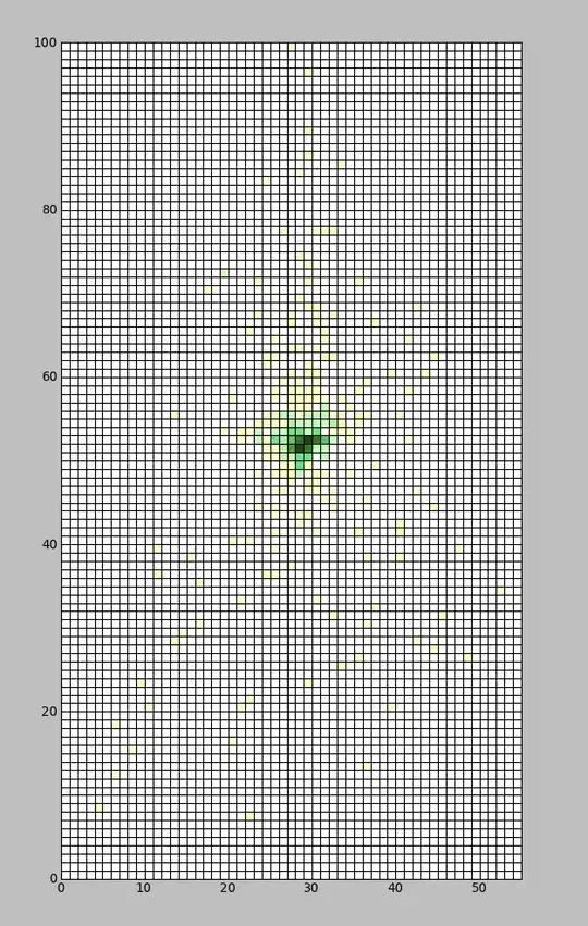
which now deskewed the colors!! we have basically created a symmetric in appearance color bar. Even if our numbers are far from symmetric.
Ok, I know that was a TON to read and digest. but here are the main takeaways this code
- uses full 3-color conditional formatting (not simply setting the two extreme colors the same to look like abs value)
- creates symmetric color ranges by using a obstructed cell (say under a button) to hold the extreme values
- uses statistical analysis to match the color gradients even in skewed data sets
both steps are necessary and neither one on its own is sufficient to create a true mirror color scale
Since this solution requires statistical analysis of the data set, you would need to run it again any time you changed a number (which was actually the case before, I just never said it)
and now the code. Put it in vba or some other highlighting program. It is nearly impossible to read as is ..... takes deep breath
Sub main()
    Dim Rng As Range
    Dim Cell_under_button As String

    Set Rng = Range("A1:H10") 'change me!!!!!!!
    Cell_under_button = "A15"

    Call AbsoluteValColorBars(Rng, Cell_under_button)

End Sub

Function iGetPercentileFromNumber(my_range As Range, num_to_find As Double)
    If (my_range.Count <= 0) Then
        Exit Function
    End If

    Dim dval_arr() As Double
    'this is one bigger than the range becasue we will add "num_to_find" to it
    ReDim dval_arr(my_range.Count + 1)
    Dim icurr_idx As Integer
    Dim ipos_num As Integer

    icurr_idx = 0

    'creates array of all the numbers in your range
    For Each cell In my_range
        dval_arr(icurr_idx) = cell.Value
        icurr_idx = icurr_idx + 1
    Next

    'adds the number we are searching for to the array
    dval_arr(icurr_idx) = num_to_find

    'sorts array in descending order
    dval_arr = BubbleSrt(dval_arr, False)

    'if match_type is 0, MATCH finds an exact match
    ipos_exact = Application.Match(CLng(num_to_find), dval_arr, 0)

    'there is a runtime error that can crop up when num_to_find isn't formated as long
    'so we converted it, if it was a double we may not find an exact match so ipos_Exact
    'may fail. now we have to find the closest numbers below or above clong(num_to_find)
    'If match_type is -1, MATCH finds the value <= num_to_find
    ipos_small = Application.Match(CLng(num_to_find), dval_arr, -1)

    If (IsError(ipos_small)) Then
        Exit Function
    End If

    'sorts array in ascending order
    dval_arr = BubbleSrt(dval_arr, True)

    'now we find the index of our  mid color point
    'If match_type is 1, MATCH finds the value >= num_to_find
    ipos_large = Application.Match(CLng(num_to_find), dval_arr, 1)

    If (IsError(ipos_large)) Then
        Exit Function
    End If

    'barring any crazy errors descending order = reverse order (ascending) so
    ipos_small = UBound(dval_arr) - ipos_small

    'to minimize color error we pick the value closest to num_to_find
    If Not (IsError(ipos_exact)) Then
        'barring any crazy errors descending order = reverse order (ascending) so
        'since the index was WRT descending subtract that from the length to get ascending
        ipos_num = UBound(dval_arr) - ipos_exact
    Else
        If (Abs(dval_arr(ipos_large) - num_to_find) < Abs(dval_arr(ipos_small) - num_to_find)) Then
            ipos_num = ipos_large
        Else
            ipos_num = ipos_small
        End If
    End If

    'gets the percentile as an integer value 0-100
    iGetPercentileFromNumber = Round(CDbl(ipos_num) / my_range.Count * 100)
End Function

'fairly well known algorithm doesn't need muxh explanation
Public Function BubbleSrt(ArrayIn, Ascending As Boolean)
    Dim SrtTemp As Variant
    Dim i As Long
    Dim j As Long


    If Ascending = True Then
        For i = LBound(ArrayIn) To UBound(ArrayIn)
             For j = i + 1 To UBound(ArrayIn)
                 If ArrayIn(i) > ArrayIn(j) Then
                     SrtTemp = ArrayIn(j)
                     ArrayIn(j) = ArrayIn(i)
                     ArrayIn(i) = SrtTemp
                 End If
             Next j
         Next i
    Else
        For i = LBound(ArrayIn) To UBound(ArrayIn)
             For j = i + 1 To UBound(ArrayIn)
                 If ArrayIn(i) < ArrayIn(j) Then
                     SrtTemp = ArrayIn(j)
                     ArrayIn(j) = ArrayIn(i)
                     ArrayIn(i) = SrtTemp
                 End If
             Next j
         Next i
    End If

    BubbleSrt = ArrayIn
End Function

Sub AbsoluteValColorBars(Rng As Range, Cell_under_button As String)
    negrange = ""
    posrange = ""

    'deletes existing rules
    Rng.FormatConditions.Delete

    'makes a negative and positive range
    For Each cell In Rng
        If cell.Value < 0 Then
            ' im certain there is a better way to get the column character
            negrange = negrange & Chr(cell.Column + 64) & cell.Row & ","
        Else
            ' im certain there is a better way to get the column character
            posrange = posrange & Chr(cell.Column + 64) & cell.Row & ","
        End If
    Next cell

    'removes trailing comma
    If Len(negrange) > 0 Then
        negrange = Left(negrange, Len(negrange) - 1)
    End If

    If Len(posrange) > 0 Then
        posrange = Left(posrange, Len(posrange) - 1)
    End If

    'finds the data extrema
    most_pos = WorksheetFunction.Max(Range(posrange))
    most_neg = WorksheetFunction.Min(Range(negrange))

    'initial values
    neg_range_percentile = 50
    pos_range_percentile = 50

    'if the negative range has the most extreme value
    If (most_pos + most_neg < 0) Then
        'put the corresponding positive number in our obstructed cell
        Range(Cell_under_button).Value = -1 * most_neg
        'and add it to the positive range, to reskew the data
        posrange = posrange & "," & Cell_under_button

        'gets the 50th percentile number from neg range and tries to mirror it in pos range
        'this should statistically skew the data
        the_num = WorksheetFunction.Percentile_Inc(Range(negrange), 0.5)
        pos_range_percentile = iGetPercentileFromNumber(Range(posrange), -1 * the_num)
    Else
        'put the corresponding negative number in our obstructed cell
        Range(Cell_under_button).Value = -1 * most_pos
        'and add it to the positive range, to reskew the data
        negrange = negrange & "," & Cell_under_button

        'gets the 50th percentile number from pos range and tries to mirror it in neg range
        'this should statistically skew the data
        the_num = WorksheetFunction.Percentile_Inc(Range(posrange), 0.5)
        neg_range_percentile = iGetPercentileFromNumber(Range(negrange), -1 * the_num)
    End If

    'low red high green for positive range
    Call addColorBar(posrange, False, pos_range_percentile)

     'high red low green for negative range
    Call addColorBar(negrange, True, neg_range_percentile)

End Sub
Sub addColorBar(my_range, binverted, imidcolorpercentile)
    If (binverted) Then
        'ai -> array ints
        adcolor = Array(8109667, 8711167, 7039480)
        '               green  , yellow , red
    Else
        adcolor = Array(7039480, 8711167, 8109667)
        '               red    , yellow , greeb
    End If

    Range(my_range).Select

     'these were just found using the record macro feature
    Selection.FormatConditions.AddColorScale ColorScaleType:=3
    Selection.FormatConditions(Selection.FormatConditions.Count).SetFirstPriority

    'assigns a color for the lowest values in the range
    Selection.FormatConditions(1).ColorScaleCriteria(1).Type = _
        xlConditionValueLowestValue
    With Selection.FormatConditions(1).ColorScaleCriteria(1).FormatColor
        .Color = adcolor(0)
        .TintAndShade = 0
    End With

    'assigns color to... midpoint of range
    Selection.FormatConditions(1).ColorScaleCriteria(2).Type = _
        xlConditionValuePercentile
    Selection.FormatConditions(1).ColorScaleCriteria(2).Value = imidcolorpercentile 'originally 50
    With Selection.FormatConditions(1).ColorScaleCriteria(2).FormatColor
        .Color = adcolor(1)
        .TintAndShade = 0
    End With

    'assigns colors to highest values in the range
    Selection.FormatConditions(1).ColorScaleCriteria(3).Type = _
        xlConditionValueHighestValue
    With Selection.FormatConditions(1).ColorScaleCriteria(3).FormatColor
        .Color = adcolor(2)
        .TintAndShade = 0
    End With
End Sub