Algorithm to group sets of points together that follow a direction

Question

Note: I am placing this question in both the MATLAB and Python tags as I am the most proficient in these languages. However, I welcome solutions in any language.

---

Question Preamble

I have taken an image with a fisheye lens. This image consists of a pattern with a bunch of square objects. What I want to do with this image is detect the centroid of each of these squares, then use these points to perform an undistortion of the image - specifically, I am seeking the right distortion model parameters. It should be noted that not all of the squares need to be detected. As long as a good majority of them are, then that's totally fine.... but that isn't the point of this post. The parameter estimation algorithm I have already written, but the problem is that it requires points that appear collinear in the image.

The base question I want to ask is given these points, what is the best way to group them together so that each group consists of a horizontal line or vertical line?

Background to my problem

This isn't really important with regards to the question I'm asking, but if you'd like to know where I got my data from and to further understand the question I'm asking, please read. If you're not interested, then you can skip right to the Problem setup section below.

---

An example of an image I am dealing with is shown below:

It is a 960 x 960 image. The image was originally higher resolution, but I subsample the image to facilitate faster processing time. As you can see, there are a bunch of square patterns that are dispersed in the image. Also, the centroids I have calculated are with respect to the above subsampled image.

The pipeline I have set up to retrieve the centroids is the following:

1. Perform a Canny Edge Detection
2. Focus on a region of interest that minimizes false positives. This region of interest is basically the squares without any of the black tape that covers one of their sides.
3. Find all distinct closed contours

4. For each distinct closed contour...

   a. Perform a Harris Corner Detection

   b. Determine if the result has 4 corner points

   c. If this does, then this contour belonged to a square and find the centroid of this shape

   d. If it doesn't, then skip this shape

5. Place all detected centroids from Step #4 into a matrix for further examination.

Here's an example result with the above image. Each detected square has the four points colour coded according to the location of where it is with respect to the square itself. For each centroid that I have detected, I write an ID right where that centroid is in the image itself.

With the above image, there are 37 detected squares.

Problem Setup

Suppose I have some image pixel points stored in a N x 3 matrix. The first two columns are the x (horizontal) and y (vertical) coordinates where in image coordinate space, the y coordinate is inverted, which means that positive y moves downwards. The third column is an ID associated with the point.

Here is some code written in MATLAB that takes these points, plots them onto a 2D grid and labels each point with the third column of the matrix. If you read the above background, these are the points that were detected by my algorithm outlined above.

data = [ 475.  ,  605.75,    1.;
       571.  ,  586.5 ,    2.;
       233.  ,  558.5 ,    3.;
       669.5 ,  562.75,    4.;
       291.25,  546.25,    5.;
       759.  ,  536.25,    6.;
       362.5 ,  531.5 ,    7.;
       448.  ,  513.5 ,    8.;
       834.5 ,  510.  ,    9.;
       897.25,  486.  ,   10.;
       545.5 ,  491.25,   11.;
       214.5 ,  481.25,   12.;
       271.25,  463.  ,   13.;
       646.5 ,  466.75,   14.;
       739.  ,  442.75,   15.;
       340.5 ,  441.5 ,   16.;
       817.75,  421.5 ,   17.;
       423.75,  417.75,   18.;
       202.5 ,  406.  ,   19.;
       519.25,  392.25,   20.;
       257.5 ,  382.  ,   21.;
       619.25,  368.5 ,   22.;
       148.  ,  359.75,   23.;
       324.5 ,  356.  ,   24.;
       713.  ,  347.75,   25.;
       195.  ,  335.  ,   26.;
       793.5 ,  332.5 ,   27.;
       403.75,  328.  ,   28.;
       249.25,  308.  ,   29.;
       495.5 ,  300.75,   30.;
       314.  ,  279.  ,   31.;
       764.25,  249.5 ,   32.;
       389.5 ,  249.5 ,   33.;
       475.  ,  221.5 ,   34.;
       565.75,  199.  ,   35.;
       802.75,  173.75,   36.;
       733.  ,  176.25,   37.];

figure; hold on;
axis ij;
scatter(data(:,1), data(:,2),40, 'r.');
text(data(:,1)+10, data(:,2)+10, num2str(data(:,3)));

Similarly in Python, using numpy and matplotlib, we have:

import numpy as np
import matplotlib.pyplot as plt

data = np.array([[ 475.  ,  605.75,    1.  ],
   [ 571.  ,  586.5 ,    2.  ],
   [ 233.  ,  558.5 ,    3.  ],
   [ 669.5 ,  562.75,    4.  ],
   [ 291.25,  546.25,    5.  ],
   [ 759.  ,  536.25,    6.  ],
   [ 362.5 ,  531.5 ,    7.  ],
   [ 448.  ,  513.5 ,    8.  ],
   [ 834.5 ,  510.  ,    9.  ],
   [ 897.25,  486.  ,   10.  ],
   [ 545.5 ,  491.25,   11.  ],
   [ 214.5 ,  481.25,   12.  ],
   [ 271.25,  463.  ,   13.  ],
   [ 646.5 ,  466.75,   14.  ],
   [ 739.  ,  442.75,   15.  ],
   [ 340.5 ,  441.5 ,   16.  ],
   [ 817.75,  421.5 ,   17.  ],
   [ 423.75,  417.75,   18.  ],
   [ 202.5 ,  406.  ,   19.  ],
   [ 519.25,  392.25,   20.  ],
   [ 257.5 ,  382.  ,   21.  ],
   [ 619.25,  368.5 ,   22.  ],
   [ 148.  ,  359.75,   23.  ],
   [ 324.5 ,  356.  ,   24.  ],
   [ 713.  ,  347.75,   25.  ],
   [ 195.  ,  335.  ,   26.  ],
   [ 793.5 ,  332.5 ,   27.  ],
   [ 403.75,  328.  ,   28.  ],
   [ 249.25,  308.  ,   29.  ],
   [ 495.5 ,  300.75,   30.  ],
   [ 314.  ,  279.  ,   31.  ],
   [ 764.25,  249.5 ,   32.  ],
   [ 389.5 ,  249.5 ,   33.  ],
   [ 475.  ,  221.5 ,   34.  ],
   [ 565.75,  199.  ,   35.  ],
   [ 802.75,  173.75,   36.  ],
   [ 733.  ,  176.25,   37.  ]])

plt.figure()
plt.gca().invert_yaxis()

plt.plot(data[:,0], data[:,1], 'r.', markersize=14)

for idx in np.arange(data.shape[0]):
    plt.text(data[idx,0]+10, data[idx,1]+10, str(int(data[idx,2])), size='large')

plt.show()

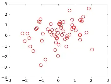
We get:

---

Back to the question

As you can see, these points are more or less in a grid pattern and you can see that we can form lines between the points. Specifically, you can see that there are lines that can be formed horizontally and vertically.

For example, if you reference the image in the background section of my problem, we can see that there are 5 groups of points that can be grouped in a horizontal manner. For example, points 23, 26, 29, 31, 33, 34, 35, 37 and 36 form one group. Points 19, 21, 24, 28, 30 and 32 form another group and so on and so forth. Similarly in a vertical sense, we can see that points 26, 19, 12 and 3 form one group, points 29, 21, 13 and 5 form another group and so on.

---

Question to ask

My question is this: What is a method that can successfully group points in horizontal groupings and vertical groupings separately, given that the points could be in any orientation?

Conditions

1. There must be at least three points per line. If there is anything less than that, then this does not qualify as a segment. Therefore, the points 36 and 10 don't qualify as a vertical line, and similarly the isolated point 23 shouldn't quality as a vertical line, but it is part of the first horizontal grouping.

2. The above calibration pattern can be in any orientation. However, for what I'm dealing with, the worst kind of orientation you can get is what you see above in the background section.

---

Expected Output

The output would be a pair of lists where the first list has elements where each element gives you a sequence of point IDs that form a horizontal line. Similarly, the second list has elements where each element gives you a sequence of point IDs that form a vertical line.

Therefore, the expected output for the horizontal sequences would look something like this:

MATLAB

horiz_list = {[23, 26, 29, 31, 33, 34, 35, 37, 36], [19, 21, 24, 28, 30, 32], ...};
vert_list = {[26, 19, 12, 3], [29, 21, 13, 5], ....};

Python

horiz_list = [[23, 26, 29, 31, 33, 34, 35, 37, 36], [19, 21, 24, 28, 30, 32], ....]
vert_list = [[26, 19, 12, 3], [29, 21, 13, 5], ...]

What I have tried

Algorithmically, what I have tried is to undo the rotation that is experienced at these points. I've performed Principal Components Analysis and I tried projecting the points with respect to the computed orthogonal basis vectors so that the points would more or less be on a straight rectangular grid.

Once I have that, it's just a simple matter of doing some scanline processing where you could group points based on a differential change on either the horizontal or vertical coordinates. You'd sort the coordinates by either the x or y values, then examine these sorted coordinates and look for a large change. Once you encounter this change, then you can group points in between the changes together to form your lines. Doing this with respect to each dimension would give you either the horizontal or vertical groupings.

With regards to PCA, here's what I did in MATLAB and Python:

MATLAB

%# Step #1 - Get just the data - no IDs
data_raw = data(:,1:2);

%# Decentralize mean
data_nomean = bsxfun(@minus, data_raw, mean(data_raw,1));

%# Step #2 - Determine covariance matrix
%# This already decentralizes the mean
cov_data = cov(data_raw);

%# Step #3 - Determine right singular vectors
[~,~,V] = svd(cov_data);

%# Step #4 - Transform data with respect to basis
F = V.'*data_nomean.';

%# Visualize both the original data points and transformed data
figure;
plot(F(1,:), F(2,:), 'b.', 'MarkerSize', 14);
axis ij;
hold on;
plot(data(:,1), data(:,2), 'r.', 'MarkerSize', 14);

Python

import numpy as np
import numpy.linalg as la

# Step #1 and Step #2 - Decentralize mean
centroids_raw = data[:,:2]
mean_data = np.mean(centroids_raw, axis=0)

# Transpose for covariance calculation
data_nomean = (centroids_raw - mean_data).T

# Step #3 - Determine covariance matrix
# Doesn't matter if you do this on the decentralized result
# or the normal result - cov subtracts the mean off anyway
cov_data = np.cov(data_nomean)

# Step #4 - Determine right singular vectors via SVD
# Note - This is already V^T, so there's no need to transpose
_,_,V = la.svd(cov_data)

# Step #5 - Transform data with respect to basis
data_transform = np.dot(V, data_nomean).T

plt.figure()
plt.gca().invert_yaxis()

plt.plot(data[:,0], data[:,1], 'b.', markersize=14)
plt.plot(data_transform[:,0], data_transform[:,1], 'r.', markersize=14)

plt.show()

---

The above code not only reprojects the data, but it also plots both the original points and the projected points together in a single figure. However, when I tried reprojecting my data, this is the plot I get:

The points in red are the original image coordinates while the points in blue are reprojected onto the basis vectors to try and remove the rotation. It still doesn't quite do the job. There is still some orientation with respect to the points so if I tried to do my scanline algorithm, points from the lines below for horizontal tracing or to the side for vertical tracing would be inadvertently grouped and this isn't correct.

---

Perhaps I'm overthinking the problem, but any insights you have regarding this would be greatly appreciated. If the answer is indeed superb, I would be inclined to award a high bounty as I've been stuck on this problem for quite some time.

I hope this question wasn't long winded. If you don't have an idea of how to solve this, then I thank you for your time in reading my question regardless.

Looking forward to any insights that you may have. Thanks very much!

Answer 1

Note 1: It has a number of settings -> which for other images may need to altered to get the result you want see % Settings - play around with these values

Note 2: It doesn't find all of the lines you want -> but its a starting point....

To call this function, invoke this in the command prompt:

>> [h, v] = testLines;

We get:

>> celldisp(h)

h{1} =
     1     2     4     6     9    10
h{2} =
     3     5     7     8    11    14    15    17
h{3} =
     1     2     4     6     9    10
h{4} =
     3     5     7     8    11    14    15    17
h{5} =
     1     2     4     6     9    10
h{6} =
     3     5     7     8    11    14    15    17
h{7} =
     3     5     7     8    11    14    15    17
h{8} =
     1     2     4     6     9    10
h{9} =
     1     2     4     6     9    10
h{10} =
    12    13    16    18    20    22    25    27
h{11} =
    13    16    18    20    22    25    27
h{12} =
     3     5     7     8    11    14    15    17
h{13} =
     3     5     7     8    11    14    15
h{14} =
    12    13    16    18    20    22    25    27
h{15} =
     3     5     7     8    11    14    15    17
h{16} =
    12    13    16    18    20    22    25    27
h{17} =
    19    21    24    28    30
h{18} =
    21    24    28    30
h{19} =
    12    13    16    18    20    22    25    27
h{20} =
    19    21    24    28    30
h{21} =
    12    13    16    18    20    22    24    25
h{22} =
    12    13    16    18    20    22    24    25    27
h{23} =
    23    26    29    31    33    34    35
h{24} =
    23    26    29    31    33    34    35    37
h{25} =
    23    26    29    31    33    34    35    36    37
h{26} =
    33    34    35    37    36
h{27} =
    31    33    34    35    37

>> celldisp(v)
v{1} =
    33    28    18     8     1
v{2} =
    34    30    20    11     2
v{3} =
    26    19    12     3
v{4} =
    35    22    14     4
v{5} =
    29    21    13     5
v{6} =
    25    15     6
v{7} =
    31    24    16     7
v{8} =
    37    32    27    17     9

A figure is also generated that draws the lines through each proper set of points:

function [horiz_list, vert_list] = testLines

global counter;
global colours; 
close all;

data = [ 475.  ,  605.75,    1.;
       571.  ,  586.5 ,    2.;
       233.  ,  558.5 ,    3.;
       669.5 ,  562.75,    4.;
       291.25,  546.25,    5.;
       759.  ,  536.25,    6.;
       362.5 ,  531.5 ,    7.;
       448.  ,  513.5 ,    8.;
       834.5 ,  510.  ,    9.;
       897.25,  486.  ,   10.;
       545.5 ,  491.25,   11.;
       214.5 ,  481.25,   12.;
       271.25,  463.  ,   13.;
       646.5 ,  466.75,   14.;
       739.  ,  442.75,   15.;
       340.5 ,  441.5 ,   16.;
       817.75,  421.5 ,   17.;
       423.75,  417.75,   18.;
       202.5 ,  406.  ,   19.;
       519.25,  392.25,   20.;
       257.5 ,  382.  ,   21.;
       619.25,  368.5 ,   22.;
       148.  ,  359.75,   23.;
       324.5 ,  356.  ,   24.;
       713.  ,  347.75,   25.;
       195.  ,  335.  ,   26.;
       793.5 ,  332.5 ,   27.;
       403.75,  328.  ,   28.;
       249.25,  308.  ,   29.;
       495.5 ,  300.75,   30.;
       314.  ,  279.  ,   31.;
       764.25,  249.5 ,   32.;
       389.5 ,  249.5 ,   33.;
       475.  ,  221.5 ,   34.;
       565.75,  199.  ,   35.;
       802.75,  173.75,   36.;
       733.  ,  176.25,   37.];

figure; hold on;
axis ij;

% Change due to Benoit_11
scatter(data(:,1), data(:,2),40, 'r.'); text(data(:,1)+10, data(:,2)+10, num2str(data(:,3)));
text(data(:,1)+10, data(:,2)+10, num2str(data(:,3)));

% Process your data as above then run the function below(note it has sub functions)
counter = 0;
colours = 'bgrcmy';
[horiz_list, vert_list] = findClosestPoints ( data(:,1), data(:,2) );


function [horiz_list, vert_list] = findClosestPoints ( x, y )
  % calc length of points
  nX = length(x);
  % set up place holder flags
  modelledH = false(nX,1);
  modelledV = false(nX,1);
  horiz_list = {};
  vert_list = {};

  % loop for all points
  for p=1:nX
    % have we already modelled a horizontal line through these?
    % second last param - true - horizontal, false - vertical
    if modelledH(p)==false
      [modelledH, index] = ModelPoints ( p, x, y, modelledH, true, true );
      horiz_list = [horiz_list index];
    else
      [~, index] = ModelPoints ( p, x, y, modelledH, true, false );
      horiz_list = [horiz_list index];
    end

    % make a temp copy of the x and y and remove any of the points modelled 
    %  from the horizontal -> this  is to avoid them being found in the 
    %  second call.
    tempX = x;
    tempY = y;
    tempX(index) = NaN;
    tempY(index) = NaN;
    tempX(p) = x(p);
    tempY(p) = y(p);
    % Have we found a vertial line?
    if modelledV(p)==false
      [modelledV, index] = ModelPoints ( p, tempX, tempY, modelledV, false, true );
      vert_list = [vert_list index];
    end
  end
end
function [modelled, index] = ModelPoints ( p, x, y, modelled, method, fullRun )
  % p - row in your original data matrix
  % x - data(:,1)
  % y - data(:,2)
  % modelled - array of flags to whether rows have been modelled
  % method   - horizontal or vertical (used to calc graadients)
  % fullRun  - full calc or just to get indexes 
  %            this could be made better by storing the indexes of each horizontal in the method above

  % Settings - play around with these values 
  gradDelta = 0.2;  % find points where gradient is less than this value
  gradLimit = 0.45; % if mean gradient of line is above this ignore
  numberOfPointsToCheck = 7; % number of points to check when look along the line
                        % to find other points (this reduces chance of it
                        % finding other points far away
                        %  I optimised this for your example to be 7
                        %  Try varying it and you will see how it effect the result.

  % Find the index of points which are inline.
  [index, grad] = CalcIndex ( x, y, p, gradDelta, method );
  % check gradient of line
  if abs(mean(grad))>gradLimit
    index = [];
    return
  end
  % add point of interest to index
  index = [p index];

  % loop through all points found above to find any other points which are in
  %  line with these points (this allows for slight curvature
  combineIndex = [];
  for ii=2:length(index)
    % Find inedex of the points found above (find points on curve)
    [index2] = CalcIndex ( x, y, index(ii), gradDelta, method, numberOfPointsToCheck, grad(ii-1) );

    % Check that the point on this line are on the original (i.e. inline -> not at large angle
    if any(ismember(index,index2))
      % store points found
      combineIndex = unique([index2 combineIndex]);
    end
  end

  % copy to index
  index = combineIndex;
  if fullRun
    %  do some plotting
    %  TODO: here you would need to calculate your arrays to output.
    xx = x(index);
    [sX,sOrder] = sort(xx);
    % Check its found at least 3 points
    if length ( index(sOrder) ) > 2
      % flag the modelled on the points found
      modelled(index(sOrder)) = true;
      % plot the data
      plot ( x(index(sOrder)), y(index(sOrder)), colours(mod(counter,numel(colours)) + 1));
      counter = counter + 1;
    end
    index = index(sOrder);
  end
end  
function [index, gradCheck] = CalcIndex ( x, y, p, gradLimit, method, nPoints2Consider, refGrad )
  % x - data(:,1)
  % y - data(:,2)
  % p - point of interest
  % method (x/y) or (y\x)
  % nPoints2Consider - only look at N points (options)
  % refgrad          - rather than looking for gradient of closest point -> use this
  %                  - reference gradient to find similar points (finds points on curve)
  nX = length(x);
  % calculate gradient
  for g=1:nX
    if method
      grad(g) = (x(g)-x(p))\(y(g)-y(p));
    else
      grad(g) = (y(g)-y(p))\(x(g)-x(p));
    end
  end
  % find distance to all other points
  delta = sqrt ( (x-x(p)).^2 + (y-y(p)).^2 );
  % set its self = NaN
  delta(delta==min(delta)) = NaN;
  % find the closest points
  [m,order] = sort(delta);

  if nargin == 7
    % for finding along curve
    % set any far away points to be NaN
    grad(order(nPoints2Consider+1:end)) = NaN;
    % find the closest points to the reference gradient within the allowable limit
    index = find(abs(grad-refGrad)<gradLimit==1);
    % store output
    gradCheck = grad(index);
  else
    % find the points which are closes to the gradient of the closest point
    index = find(abs(grad-grad(order(1)))<gradLimit==1);
    % store gradients to output
    gradCheck = grad(index);
  end
end
end

Answer 2

While I can not suggest a better approach to group any given list of centroid points than the one you already tried, I hope the following idea might help you out:

Since you are very specific about the content of your image (containing a field of squares) I was wondering if you in fact need to group the centroid points from the data given in your problem setup, or if you can use the data described in Background to the problem as well. Since you already determined the corners of each detected square as well as their position in that given square it seems to me like it would be very accurate to determine a neighbour of a given square by comparing the corner-coordinates.

So for finding any candidate for a right neighbour of any square, i would suggest you compare the upper right and lower right corner of that square with the upper left and lower left corner of any other square (or any square within a certain distance). Allowing for only small vertical differences and slightly greater horizontal differences, you can "match" two squares, if both their corresponding corner-points are close enough together.

By using an upper limit to the allowed vertical/horizontal difference between corners, you might even be able to just assign the best matching square within these boundaries as neighbour

A problem might be that you don't detect all the squares, so there is a rather large space between square 30 and 32. Since you said you need 'at least' 3 squares per row, it might be viable for you to simply ignore square 32 in that horizontal line. If that is not an option for you, you could try to match as many squares as possible and afterwards assign the "missing" squares to a point in your grid by using the previously calculated data:

In the example about square 32 you would've detected that it has upper and lower neighbours 27 and 37. Also you should've been able to determine that square 27 lies within row 1 and 37 lies within row 3, so you can assign square 32 to the "best matching" row in between, which is obviously 2 in this case.

This general approach is basically the approach you have tried already, but should hopefully be a lot more accurate since you are now comparing orientation and distance of two lines instead of simply comparing the location of two points in a grid.

Also as a sidenode on your previous attempts - can you use the black cornerlines to correct the initial rotation of your image a bit? This might make further distortion algorithms (like the ones that you discussed with knedlsepp in the comments) a lot more accurate. (EDIT: I did read the comments of Parag just now - comparing the points by the angle of the lines is of course basically the same as rotating the Image beforehand)

Answer 3

I'm using a cropped version of the posted image as the input. Here I'm only addressing the case where the orientation of the grid can be thought of as near horizontal/vertical. This may not fully address your scope, but I think it may give you some pointers.

Binarize the image so that the distorted squares are filled. Here I use a simple Otsu thresholding. Then take the distance transform of this binary image.

In the distance transformed image we see the gaps between the squares as peaks.

To get horizontally oriented lines, take the local maxima of each of the columns of the distance image and then find connected components.

To get vertically oriented lines, take the local maxima of each of the rows of the distance image and then find connected components.

Images below show the horizontal and vertical lines thus found with corner points as circles.

For reasonably long connected components, you can fit a curve (a line or a polynomial) and then classify the corner points, say based on the distance to the curve, on which side of the curve the point is, etc.

I did this in Matlab. I didn't try the curve fitting and classification parts.

clear all;
close all;

im = imread('0RqUd-1.jpg');
gr = rgb2gray(im);
% any preprocessing to get a binary image that fills the distorted squares
bw = ~im2bw(gr, graythresh(gr));

di = bwdist(bw);                % distance transform
di2 = imdilate(di, ones(3));    % propagate max

corners = corner(gr);           % simple corners

% find regional max for each column of dist image
regmxh = zeros(size(di2));
for c = 1:size(di2, 2)
    regmxh(:, c) = imregionalmax(di2(:, c));
end
% label connected components
ccomph = bwlabel(regmxh, 8);

% find regional max for each row of dist image
regmxv = zeros(size(di2));
for r = 1:size(di2, 1)
    regmxv(r, :) = imregionalmax(di2(r, :));
end
% label connected components
ccompv = bwlabel(regmxv, 8);

figure, imshow(gr, [])
hold on
plot(corners(:, 1), corners(:, 2), 'ro')
figure, imshow(di, [])
figure, imshow(label2rgb(ccomph), [])
hold on
plot(corners(:, 1), corners(:, 2), 'ro')
figure, imshow(label2rgb(ccompv), [])
hold on
plot(corners(:, 1), corners(:, 2), 'ro')

To get these lines for arbitrary oriented grids, you can think of the distance image as a graph and find optimal paths. See here for a nice graph based approach.