Simulink simulation behaving massively different than the same simulation using rk4

Question

I have difficulties simulating an object discribed by the following state space equations in simulink:

The right hand side of the state space equation is described by the funcion below.

function dxdt = RHS( t, x, F)
% parameters
b = 1.22;          % cart friction coeffitient 
c = 0.0027;           %pendulum friction coeffitient
g = 9.81;           % gravity
M = 0.548+0.022*2; % cart weight
m = 0.031*2; %pendulum masses
I = 0.046;%0.02*0.025/12+0.02*0.12^2+0.011*0.42^2; % moment of inertia
l = 0.1313;
% x(1) = theta
% x(2) = theta_dot
% x(3) = x
% x(4) = x_dot


dxdt = [x(2);
    (-(M+m)*c*x(2)-(M+m)*g*l*sin(x(1))-m^2*l^2*x(2)^2*sin(x(1))*cos(x(1))+m*l*b*x(4)*cos(x(1))-m*l*cos(x(1))*F)/(I*(m+M)+m*M*l^2+m^2*l^2*sin(x(1))^2);
    x(4);
    (F - b*x(4) + l*m*x(2)^2*sin(x(1)) + (l*m*cos(x(1))*(c*x(2)*(M + m) + g*l*sin(x(1))*(M + m) + F*l*m*cos(x(1)) + l^2*m^2*x(2)^2*cos(x(1))*sin(x(1)) - b*l*m*x(4)*cos(x(1))))/(I*(M + m) + l^2*m^2*sin(x(1))^2 + M*l^2*m))/(M + m)];
end

The coresponding rk4 function with a simple visualisation is shown below.

function [wi, ti] = rk4 ( RHS, t0, x0, tf, N )

%RK4 approximate the solution of the initial value problem
%
% x'(t) = RHS( t, x ), x(t0) = x0
%
% using the classical fourth-order Runge-Kutta method - this 
% routine will work for a system of first-order equations as 
% well as for a single equation
%
% calling sequences:
% [wi, ti] = rk4 ( RHS, t0, x0, tf, N )
% rk4 ( RHS, t0, x0, tf, N )
%
% inputs:
% RHS string containing name of m-file defining the 
% right-hand side of the differential equation; the
% m-file must take two inputs - first, the value of
% the independent variable; second, the value of the
% dependent variable
% t0 initial value of the independent variable
% x0 initial value of the dependent variable(s)
% if solving a system of equations, this should be a 
% row vector containing all initial values
% tf final value of the independent variable
% N number of uniformly sized time steps to be taken to
% advance the solution from t = t0 to t = tf
%
% output:
% wi vector / matrix containing values of the approximate 
% solution to the differential equation
% ti vector containing the values of the independent 
% variable at which an approximate solution has been
% obtained
%

% x(1) = theta
% x(2) = theta_dot
% x(3) = x
% x(4) = x_dot
t0 = 0; tf = 5; x0 = [pi/2; 0; 0; 0]; N = 400;
neqn = length ( x0 );
ti = linspace ( t0, tf, N+1 );
wi = [ zeros( neqn, N+1 ) ];
wi(1:neqn, 1) = x0';

h = ( tf - t0 ) / N;
% force
u = 0.0;

%init visualisation
h_cart = plot(NaN, NaN, 'Marker', 'square', 'color', 'red', 'LineWidth', 6);
hold on
h_pend = plot(NaN, NaN, 'bo', 'LineWidth', 3);
axis([-5 5 -5 5]);
axis manual;
xlim([-5 5]);
ylim([-5 5]);

for i = 1:N
    k1 = h * feval ( 'RHS', t0, x0, u );
    k2 = h * feval ( 'RHS', t0 + (h/2), x0 + (k1/2), u);
    k3 = h * feval ( 'RHS', t0 + h/2, x0 + k2/2, u);
    k4 = h * feval ( 'RHS', t0 + h, x0 + k3, u);
    x0 = x0 + ( k1 + 2*k2 + 2*k3 + k4 ) / 6;
    t0 = t0 + h;
    % model output
    wi(1:neqn,i+1) = x0';

    % model visualisation
    %plotting cart
    l = 2;
    set(h_cart, 'XData', x0(3), 'YData', 0, 'LineWidth', 5);
    %plotting pendulum
    %hold on;
   set(h_pend, 'XData', sin(x0(1))*l+x0(3), 'YData', -cos(x0(1))*l, 'LineWidth', 2);
   %hold off;
    % regulator
    pause(0.02);
end;

figure;
plot(ti, wi);
legend('theta', 'theta`', 'x', 'x`');

This gives realistic looking results for a pendulum on a cart.

Now to the problem. I wanted to recreate the exact same equations in simulink. I thought it is going to be as easy as creating the following simulink model. where I fill the fcn blocks with the second and fourth equation from the RHS file. Like this.

(-(M+m)*c*u(2)-(M+m)*g*l*sin(u(1))-m^2*l^2*u(2)^2*sin(u(1))*cos(u(1))+m*l*b*u(3)*cos(u(1))-m*l*cos(u(1))*u(4))/(I*(m+M)+m*M*l^2+m^2*l^2*sin(u(1))^2)

(u(5) - b*u(4) + l*m*u(2)^2*sin(u(1)) + (l*m*cos(u(1))*(c*u(2)*(M + m) + g*l*sin(u(1))*(M + m) + u(5)*l*m*cos(u(1)) + l^2*m^2*u(2)^2*cos(u(1))*sin(u(1)) - b*l*m*u(4)*cos(u(1))))/(I*(M + m) + l^2*m^2*sin(u(1))^2 + M*l^2*m))/(M + m)

The problem is this doesn't give the correct results from above, but the one below

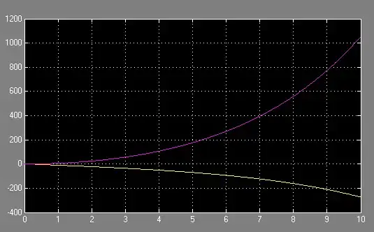
Does anybody know what I do incorrectly?

Edit:After @am304 comment I decided to add the following information. I changed the setting for the simulink solver to use the fixed-step rk4 solver, so as to get the same results. The second integrator3 from the model above has been initialized to pi/2.

Edit2: If somebody wants to check out the simulink model for themselves click on the link to download the file.

Edit3: As you can read in the answer below the problem was trivial. You can download the correct model here

Answer 1

I looked through your Simulink model and it seems you may have mixed up the two functions you were using. You used the theta_dd function where you meant to put x_dd and vice versa.

In your model, you also force x_d to be set to a constant value 0. I assume you actually meant to set the initial condition to 0, which you can see is done via the Integrator block. x_d (as an input to f) should be your state vector which is also an output of your integrators. This is just a consequence of what you define x_d to be, the integral of x_dd. This is how RK4 works as well; you use an initial state vector first and then use the predicted state vector to drive the next RK4 step.

The resulting output from the scope (i've outputted your whole state vector here) is as follows and looks like what you expect:

I do not think I should link externally to the simulink file so if you would like a copy of the file you can open a chat and ask for it. Otherwise the picture above should be sufficient enough to help you reproduce the same results.