2

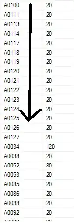
I have 4000+ rows of data need to be working on. Where column A represents the SKU, column B represents the unit and column C represents the Unit Price. The same SKU, Unit and Unit Price may duplicate at their own columns as shown as the picture attached. I need to check and highlight whether which SKU, appears to have different Unit Price but with same Unit. Which mean same SKU (Column A), same Unit (Column B) but different in Unit Price (Column C).

Is there any possible method or formula for doing this checking instead of checking row-by-row manually?

[How to I find the same cases just like row 4 in the picture (with same SKU, same Unit but different Unit Price)

How to I find the same cases just like row 4 in the picture (with same SKU, same Unit but different Unit Price?

Skyler Cheah
  • 61
  • 1
  • 2
  • 5

3 Answers3

3

You can design a Conditional Formatting rule using a formula based on the COUNTIFS function. If you set a rule such that there must be at least two other rows with the same SKU and Unit combination but with different Unit Prices then a formula can be easily derived.

First, select all of columns A:C then go to Home ► Styles ► Conditional Formatting ► New Rule. Opt for Use a formula to determine which cells to format and supply the following for the Format values where this formula is true: text box.

=AND(ROW(A1)>1, COUNTIFS($A:$A, $A1, $B:$B, $B1, $C:$C, "<>"&$C1)>1)

Click Format and apply some formatting the OK to accept the formatting and OK again to create the new rule. Your results should resemble the following.

        Conditional Formatting rogue unit prices

Note that I've added one more row of data to the sample data.

Community
  • 1
  • 1
  • There are a lot of problems with identifying the rogue unit prices; foremost would be if the OP's sample data had different unit prices for each of the original two A456's. While these can easily be found, they would also highlight any single entries. The above is just a start; I would imagine that more CF rules could be added (with different color highlighting) to identify other situations, perhaps with varying shades of red. –  Oct 08 '15 at 04:43
  • Thank you so much, this is really helpful and it works – Skyler Cheah Oct 08 '15 at 06:26
  • I am facing the problem which sometimes the data with same SKU and Unit but different Unit Price not being highlighted. And also, in my excel document, there would be like within 5 rows of data with same SKU and Unit yet different Unit Price within the 20 rows. This formula usually will highlight all the 20 rows but sometimes it missed. I do not understand why and how to fix that. – Skyler Cheah Oct 09 '15 at 05:31
  • This is simply a logic problem where conditions that match most do not always match everything desired. Additional conditions can be added but you have not provided enough details. In fact, it seems that many conditions may have to be considered. Having only seen a small sample of data, it is quite impossible to find problems in other rows that I cannot see. Please consider redacting some samples data that are causing problems to add to your original question. –  Oct 09 '15 at 06:23
0

With sorting by ColumnA, then Column B then Column C and assuming a reasonably up-to-date version of Excel, please select ColumnsA:C and HOME > Styles - Conditional Formatting, New Rule..., Use a formula to determine which cells to format and Format values where this formula is true::

=AND($A1048576=$A1,$B1048576=$B1,$C1048576<>$C1)  

Format..., select your choice of formatting (red), OK, OK.

This is a version of =AND(A2=A3,B2=B3,C2<>C3) (which follows how you expressed the problem) adapted to simplify the range selection (Applies to).

The sorting is important because this looks for the first change in Unit Price since a preceding Unit Price for the same SKU/Unit pair, consistent with your choice not to highlight [A123,5,25] though 25 is as different from 30 as 30 is from 25! In the image I have added some additional examples for illustration.

SO3006173 first example

For sorting:

SO3006173 second example

pnuts
  • 58,317
  • 11
  • 87
  • 139
  • 1
    yes, sorting is permitted. Sorry for missing your question. – Skyler Cheah Oct 08 '15 at 06:59
  • If I want to sort the data with ascending order of SKU (column A), then follow by ascending of unit (column B) then ascending for unit price (column c). Then I shall sort column C>B>A, right? But then some rows actually do not sort in order, for instance, A123 appears in row 1~20, then 350~355. So that I am not sure whether is this working or not. – Skyler Cheah Oct 09 '15 at 05:25
-1

Create a formula in column D:

=CONCATENATE(A2,"-",B2,"-",C2)

Select Column D and apply Conditonal Formatting -> Higlight Cells Rules -> Duplicate Values

Conditonal Formatting Option

Apply the formatting to unique cells.

Duplicate Values Formatting Dialog

mikek3332002
  • 3,546
  • 4
  • 37
  • 47