projectile motion simple simulation using numpy matplotlib python

Question

I am trying to graph a projectile through time at various angles. The angles range from 25 to 60 and each initial angle should have its own line on the graph. The formula for "the total time the projectile is in the air" is the formula for t. I am not sure how this total time comes into play, because I am supposed to graph the projectile at various times with various initial angles. I imagine that I would need x,x1,x2,x3,x4,x5 and the y equivalents in order to graph all six of the various angles. But I am confused on what to do about the time spent.

import numpy as np 
import matplotlib.pylab as plot 

#initialize variables 
#velocity, gravity
v = 30 
g = -9.8 
#increment theta 25 to 60 then find  t, x, y
#define x and y as arrays 
theta = np.arange(25,65,5)   

t = ((2 * v) * np.sin(theta)) / g #the total time projectile remains in the #air
t1 = np.array(t) #why are some negative 



x = ((v * t1) * np.cos(theta))
y = ((v * t1) * np.sin(theta)) - ((0.5 * g) * (t ** 2))

plot.plot(x,y)
plot.show()

Answer 1

First of all g is positive! After fixing that, let's see some equations:

You know this already, but lets take a second and discuss something. What do you need to know in order to get the trajectory of a particle?

Initial velocity and angle, right? The question is: find the position of the particle after some time given that initial velocity is v=something and theta=something. Initial is important! That's the time when we start our experiment. So time is continuous parameter! You don't need the time of flight.

One more thing: Angles can't just be written as 60, 45, etc, python needs something else in order to work, so you need to write them in numerical terms, (0,90) = (0,pi/2).

Let's see the code:

import numpy as np
import matplotlib.pylab as plot
import math as m
#initialize variables
#velocity, gravity
v = 30
g = 9.8
#increment theta 25 to 60 then find  t, x, y
#define x and y as arrays

theta = np.arange(m.pi/6, m.pi/3, m.pi/36)

t = np.linspace(0, 5, num=100) # Set time as 'continous' parameter.

for i in theta: # Calculate trajectory for every angle
    x1 = []
    y1 = []
    for k in t:
        x = ((v*k)*np.cos(i)) # get positions at every point in time
        y = ((v*k)*np.sin(i))-((0.5*g)*(k**2))
        x1.append(x)
        y1.append(y)
    p = [i for i, j in enumerate(y1) if j < 0] # Don't fall through the floor                          
    for i in sorted(p, reverse = True):
        del x1[i]
        del y1[i]

    plot.plot(x1, y1) # Plot for every angle

plot.show() # And show on one graphic

Answer 2

You are making a number of mistakes.

Firstly, less of a mistake, but matplotlib.pylab is supposedly used to access matplotlib.pyplot and numpy together (for a more matlab-like experience), I think it's more suggested to use matplotlib.pyplot as plt in scripts (see also this Q&A).

Secondly, your angles are in degrees, but math functions by default expect radians. You have to convert your angles to radians before passing them to the trigonometric functions.

Thirdly, your current code sets t1 to have a single time point for every angle. This is not what you need: you need to compute the maximum time t for every angle (which you did in t), then for each angle create a time vector from 0 to t for plotting!

Lastly, you need to use the same plotting time vector in both terms of y, since that's the solution to your mechanics problem:

y(t) = v_{0y}*t - g/2*t^2

This assumes that g is positive, which is again wrong in your code. Unless you set the y axis to point downwards, but the word "projectile" makes me think this is not the case.

So here's what I'd do:

import numpy as np 
import matplotlib.pyplot as plt 

#initialize variables 
#velocity, gravity
v = 30 
g = 9.81  #improved g to standard precision, set it to positive
#increment theta 25 to 60 then find  t, x, y
#define x and y as arrays 
theta = np.arange(25,65,5)[None,:]/180.0*np.pi #convert to radians, watch out for modulo division

plt.figure()

tmax = ((2 * v) * np.sin(theta)) / g
timemat = tmax*np.linspace(0,1,100)[:,None] #create time vectors for each angle

x = ((v * timemat) * np.cos(theta))
y = ((v * timemat) * np.sin(theta)) - ((0.5 * g) * (timemat ** 2))

plt.plot(x,y) #plot each dataset: columns of x and columns of y
plt.ylim([0,35])
plot.show()

I made use of the fact that plt.plot will plot the columns of two matrix inputs versus each other, so no loop over angles is necessary. I also used [None,:] and [:,None] to turn 1d numpy arrays to 2d row and column vectors, respectively. By multiplying a row vector and a column vector, array broadcasting ensures that the resulting matrix behaves the way we want it (i.e. each column of timemat goes from 0 to the corresponding tmax in 100 steps)

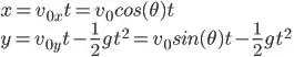
Result: