Background
When Seo and Kim ask for lambda_i, v_i <- PCA(Iycc), for i = 1, 2, 3, they want:
from numpy.linalg import eig
lambdas, vs = eig(np.dot(Izycc, Izycc.T))
for a 3×N array Izycc. That is, they want the three eigenvalues and eigenvectors of the 3×3 covariance matrix of Izycc, the 3×N array (for you, N = 500*500).
However, you almost never want to compute the covariance matrix, then find its eigendecomposition, because of numerical instability. There is a much better way to get the same lambdas, vs, using the singular value decomposition (SVD) of Izycc directly (see this answer). The code below shows you how to do this.
Just show me the code
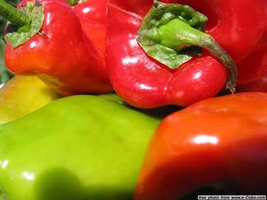
First download http://cadik.posvete.cz/color_to_gray_evaluation/img/155_5572_jpg/155_5572_jpg.jpg and save it as peppers.jpg.
Then, run the following:
import numpy as np
import cv2
from numpy.linalg import svd, norm

# Read input image
Ibgr = cv2.imread('peppers.jpg')

# Convert to YCrCb
Iycc = cv2.cvtColor(Ibgr, cv2.COLOR_BGR2YCR_CB)

# Reshape the H by W by 3 array to a 3 by N array (N = W * H)
Izycc = Iycc.reshape([-1, 3]).T

# Remove mean along Y, Cr, and Cb *separately*!
Izycc = Izycc - Izycc.mean(1)[:, np.newaxis]

# Make sure we're dealing with zero-mean data here: the mean for Y, Cr, and Cb
# should separately be zero. Recall: Izycc is 3 by N array.
assert(np.allclose(np.mean(Izycc, 1), 0.0))

# Compute data array's SVD. Ignore the 3rd return value: unimportant.
(U, S) = svd(Izycc, full_matrices=False)[:2]

# Square the data's singular vectors to get the eigenvalues. Then, normalize
# the three eigenvalues to unit norm and finally, make a diagonal matrix out of
# them. N.B.: the scaling factor of `norm(S**2)` is, I believe, arbitrary: the
# rest of the algorithm doesn't really care if/how the eigenvalues are scaled,
# since we will rescale the grayscale values to [0, 255] anyway.
eigvals = np.diag(S**2 / norm(S**2))

# Eigenvectors are just the left-singular vectors.
eigvecs = U;

# Project the YCrCb data onto the principal components and reshape to W by H
# array.
Igray = np.dot(eigvecs.T, np.dot(eigvals, Izycc)).sum(0).reshape(Iycc.shape[:2])

# Rescale Igray to [0, 255]. This is a fancy way to do this.
from scipy.interpolate import interp1d
Igray = np.floor((interp1d([Igray.min(), Igray.max()],
                            [0.0, 256.0 - 1e-4]))(Igray))

# Make sure we don't accidentally produce a photographic negative (flip image
# intensities). N.B.: `norm` is often expensive; in real life, try to see if
# there's a more efficient way to do this.
if norm(Iycc[:,:,0] - Igray) > norm(Iycc[:,:,0] - (255.0 - Igray)):
    Igray = 255 - Igray

# Display result
if True:
    import pylab
    pylab.ion()
    pylab.imshow(Igray, cmap='gray')

# Save result
cv2.imwrite('peppers-gray.png', Igray.astype(np.uint8))
This produces the following grayscale image, which seems to match the result in Figure 4 of the paper (though see caveat at the bottom of this answer!):

Errors in your implementation
Izycc = Iycc - Iycc.mean() WRONG. Iycc.mean() flattens the image and computes the mean. You want Izycc such that the Y channel, Cr channel, and Cb channel all have zero-mean. You could do this in a for dim in range(3)-loop, but I did it above with array broadcasting. I also have an assert above to make sure this condition holds. The trick where you get the eigendecomposition of the covariance matrix from the SVD of the data array requires zero-mean Y/Cr/Cb channels.
np.linalg.eig(Izycc[:,:,i]) WRONG. The contribution of this paper is to use principal components to convert color to grayscale. This means you have to combine the colors. The processing you were doing above was on a channel-by-channel basis—no combination of colors. Moreover, it was totally wrong to decompose the 500×500 array: the width/height of the array don’t matter, only pixels. For this reason, I reshape the three channels of the input into 3×whatever and operate on that matrix. Make sure you understand what’s happening after BGR-to-YCrCb conversion and before the SVD.
Not so much an error but a caution: when calling numpy.linalg.svd, the full_matrices=False keyword is important: this makes the “economy-size” SVD, calculating just three left/right singular vectors and just three singular values. The full-sized SVD will attempt to make an N×N array of right-singular vectors: with N = 114270 pixels (293 by 390 image), an N×N array of float64 will be N ** 2 * 8 / 1024 ** 3 or 97 gigabytes.
Final note
The magic of this algorithm is really in a single line from my code:
Igray = np.dot(eigvecs.T, np.dot(eigvals, Izycc)).sum(0) # .reshape...
This is where The Math is thickest, so let’s break it down.
Izycc is a 3×N array whose rows are zero-mean; eigvals is a 3×3 diagonal array containing the eigenvalues of the covariance matrix dot(Izycc, Izycc.T) (as mentioned above, computed via a shortcut, using SVD of Izycc),eigvecs is a 3×3 orthonormal matrix whose columns are the eigenvectors corresponding to those eigenvalues of that covariance.
Because these are Numpy arrays and not matrixes, we have to use dot(x,y) for matrix-matrix-multiplication, and then we use sum, and both of these obscure the linear algebra. You can check for yourself but the above calculation (before the .reshape() call) is equivalent to
np.ones([1, 3]) · eigvecs.T · eigvals · Izycc = dot([[-0.79463857, -0.18382267, 0.11589724]], Izycc)
where · is true matrix-matrix-multiplication, and the sum is replaced by pre-multiplying by a row-vector of ones. Those three numbers,
- -0.79463857 multiplying each pixels’s Y-channel (luma),
- -0.18382267 multiplying Cr (red-difference), and
- 0.11589724 multiplying Cb (blue-difference),
specify the “perfect” weighted average, for this particular image: each pixel’s Y/Cr/Cb channels are being aligned with the image’s covariance matrix and summed. Numerically speaking, each pixel’s Y-value is slightly attenuated, its Cr-value is significantly attenuated, and its Cb-value is even more attenuated but with an opposite sign—this makes sense, we expect the luma to be most informative for a grayscale so its contribution is the highest.
Minor caveat
I’m not really sure where OpenCV’s RGB to YCrCb conversion comes from. The documentation for cvtColor, specifically the section on RGB ↔︎ YCrCb JPEG doesn’t seem to correspond to any of the transforms specified on Wikipedia. When I use, say, the Colorspace Transformations Matlab package to just do the RGB to YCrCb conversion (which cites the Wikipedia entry), I get a nicer grayscale image which appears to be more similar to the paper’s Figure 4:
I’m totally out of my depth when it comes to these color transformations—if someone can explain how to get Wikipedia or Matlab’s Colorspace Transformations equivalents in Python/OpenCV, that’d be very kind. Nonetheless, this caveat is about preparing the data. After you make Izycc, the 3×N zero-mean data array, the above code fully-specifies the remaining processing.


