I want to draw a graph which is familiar to the enterotype plot in the research. But my new multiple-ggproto seems terrible as showed in p1, owing to the missing backgroup color of the label. I've tried multiple variations of this, for example modify GeomLabel$draw_panel in order to reset the default arguments of geom in ggplot2::ggproto. However, I could not find the labelGrob() function which is removed in ggplot2 and grid package. Thus, the solution of modification didn't work. How to modify the backgroup color of label in the multiple-ggproto. Any ideas? Thanks in advance. Here is my code and two pictures.
p1: the background color of label should be white or the text color should be black.

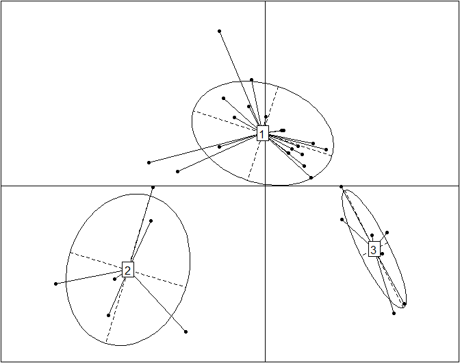
P2:displays the wrong point color, line color and legend. 
geom_enterotype <- function(mapping = NULL, data = NULL, stat = "identity",  position = "identity",
                            alpha = 0.3, prop = 0.5, ..., lineend = "butt", linejoin = "round",
                            linemitre = 1, arrow = NULL, na.rm = FALSE, parse = FALSE,
                            nudge_x = 0, nudge_y = 0, label.padding = unit(0.15, "lines"),
                            label.r = unit(0.15, "lines"), label.size = 0.1,
                            show.legend = TRUE, inherit.aes = TRUE) {
library(ggplot2)
# create new stat and geom for PCA scatterplot with ellipses
StatEllipse <- ggproto("StatEllipse", Stat,
    required_aes = c("x", "y"),
    compute_group = function(., data, scales, level = 0.75, segments = 51, ...) {
    library(MASS)
    dfn <- 2
    dfd <- length(data$x) - 1
    if (dfd < 3) {
        ellipse <- rbind(c(NA, NA))
    } else {
        v <- cov.trob(cbind(data$x, data$y))
        shape <- v$cov
        center <- v$center
        radius <- sqrt(dfn * qf(level, dfn, dfd))
        angles <- (0:segments) * 2 * pi/segments
        unit.circle <- cbind(cos(angles), sin(angles))
        ellipse <- t(center + radius * t(unit.circle %*% chol(shape)))
    }
    ellipse <- as.data.frame(ellipse)
    colnames(ellipse) <- c("x", "y")
    return(ellipse)
})

# write new ggproto
GeomEllipse <- ggproto("GeomEllipse", Geom,
    draw_group = function(data, panel_scales, coord) {
            n <- nrow(data)
            if (n == 1)
            return(zeroGrob())
            munched <- coord_munch(coord, data, panel_scales)
            munched <- munched[order(munched$group), ]
            first_idx <- !duplicated(munched$group)
            first_rows <- munched[first_idx, ]
            grid::pathGrob(munched$x, munched$y, default.units = "native",
                           id = munched$group,
                           gp = grid::gpar(col = first_rows$colour,
                           fill = alpha(first_rows$fill, first_rows$alpha), lwd = first_rows$size * .pt, lty = first_rows$linetype))
             },
             default_aes = aes(colour = "NA", fill = "grey20", size = 0.5, linetype = 1, alpha = NA, prop = 0.5),
             handle_na = function(data, params) {
                   data
           },
          required_aes = c("x", "y"),
          draw_key = draw_key_path
)

# create a new stat for PCA scatterplot with lines which totally directs to the center
StatConline <- ggproto("StatConline", Stat,
    compute_group = function(data, scales) {
    library(miscTools)
    library(MASS)
    df <- data.frame(data$x,data$y)
    mat <- as.matrix(df)
    center <- cov.trob(df)$center
    names(center)<- NULL
    mat_insert <- insertRow(mat, 2, center )
    for(i in 1:nrow(mat)) {
    mat_insert <- insertRow( mat_insert, 2*i, center )
    next
    }
    mat_insert <- mat_insert[-c(2:3),]
    rownames(mat_insert) <- NULL
    mat_insert <- as.data.frame(mat_insert,center)
    colnames(mat_insert) =c("x","y")
    return(mat_insert)
    },
    required_aes = c("x", "y")

)

# create a new stat for PCA scatterplot with center labels
StatLabel <- ggproto("StatLabel" ,Stat,
               compute_group = function(data, scales) {
                library(MASS)
                df <- data.frame(data$x,data$y)
                center <- cov.trob(df)$center
                names(center)<- NULL
                center <- t(as.data.frame(center))
                center <- as.data.frame(cbind(center))
                colnames(center) <- c("x","y")
                rownames(center) <- NULL
                return(center)
                },
                required_aes = c("x", "y")
)


layer1 <- layer(data = data, mapping = mapping, stat = stat, geom = GeomPoint,
        position = position, show.legend = show.legend, inherit.aes = inherit.aes,
        params = list(na.rm = na.rm, ...))
layer2 <- layer(stat = StatEllipse, data = data, mapping = mapping, geom = GeomEllipse, position = position, show.legend = FALSE,
                     inherit.aes = inherit.aes, params = list(na.rm = na.rm, prop = prop, alpha = alpha, ...))
layer3 <- layer(data = data, mapping = mapping, stat =  StatConline, geom = GeomPath,
                                   position = position, show.legend = show.legend, inherit.aes = inherit.aes,
                                   params = list(lineend = lineend, linejoin = linejoin,
                                   linemitre = linemitre, arrow = arrow, na.rm = na.rm, ...))
if (!missing(nudge_x) || !missing(nudge_y)) {
    if (!missing(position)) {
      stop("Specify either `position` or `nudge_x`/`nudge_y`",
           call. = FALSE)
    }
    position <- position_nudge(nudge_x, nudge_y)
  }
layer4 <- layer(data = data, mapping = mapping, stat = StatLabel, geom = GeomLabel,
        position = position, show.legend = FALSE, inherit.aes = inherit.aes,
        params = list(parse = parse, label.padding = label.padding,
                      label.r = label.r, label.size = label.size, na.rm = na.rm, ...))
return(list(layer1,layer2,layer3,layer4))
}

# data
data(Cars93, package = "MASS")
car_df <- Cars93[, c(3, 5, 13:15, 17, 19:25)]
car_df <- subset(car_df, Type == "Large" | Type == "Midsize" | Type == "Small")
x1 <- mean(car_df$Price) + 2 * sd(car_df$Price)
x2 <- mean(car_df$Price) - 2 * sd(car_df$Price)
car_df <- subset(car_df, Price > x2 | Price < x1)
car_df <- na.omit(car_df)

# Principal Component Analysis
car.pca <- prcomp(car_df[, -1], scale = T)
car.pca_pre <- cbind(as.data.frame(predict(car.pca)[, 1:2]), car_df[, 1])
colnames(car.pca_pre) <- c("PC1", "PC2", "Type")
xlab <- paste("PC1(", round(((car.pca$sdev[1])^2/sum((car.pca$sdev)^2)), 2) * 100, "%)", sep = "")
ylab <- paste("PC2(", round(((car.pca$sdev[2])^2/sum((car.pca$sdev)^2)), 2) * 100, "%)", sep = "")
head(car.pca_pre)

#plot
library(ggplot2)
p1 <- ggplot(car.pca_pre, aes(PC1, PC2, fill = Type , color= Type ,label = Type)) +
geom_enterotype()
p2 <- ggplot(car.pca_pre, aes(PC1, PC2, fill = Type , label = Type)) +
geom_enterotype()


