0

I have this 2D normal distribution defined as

mu = [0 0];
Sigma = [1 0.5^0.5; 0.5^0.5 1];

Is there a way to get the contour data when the cumulative probability say is 95%. I do not want the plot but the value of the (x,y) points that results in 95% contour.

It would be very kind if someone can help. Thanks in advance

rayryeng
  • 102,964
  • 22
  • 184
  • 193
user1612986
  • 1,373
  • 3
  • 22
  • 38
  • Please consult the duplicate. Look at Amro's answer - especially the EDIT section which talks about how to generate the points along the 95% error ellipse. – rayryeng Jun 06 '17 at 19:37
  • I could not follow the answer. The objective of the problem seems to be different. – user1612986 Jun 06 '17 at 19:46
  • 1
    The post generates the points of an ellipse around the data. It finds those points, then plots it. The edit also tells you how to do this for a 95% error ellipse. What you are seeking is just the points, not the plotting. So do everything up to but not including the plot. The duplicate is plotting this for two objects, but you only have one. Also, the line where the points are generated is: `e = bsxfun(@plus, VV*e, Mu');`. `e` will thus be a two column matrix where each column is a coordinate (`x` or `y`) of the points along the ellipse. – rayryeng Jun 06 '17 at 19:48
  • still it is not clear. not sure how "STD = 2; conf = 2*normcdf(STD)-1;" generate the 95% cumProb that I was looking for. It would be kind of you to give me the steps. something is strange. the contour what i will have in the end is not an ellipse. kind of different from the problem altogether. – user1612986 Jun 06 '17 at 20:28
  • You can follow this post: http://www.visiondummy.com/2014/04/draw-error-ellipse-representing-covariance-matrix/. There is sample MATLAB code you can download that will find the points for you, but it's really the same as the duplicate. – rayryeng Jun 06 '17 at 20:36
  • is it the same problem we are discussing ? You see the cumulative probability contour is not an ellipse. it is some kind of rectangular open ended region (maybe like a hyperbola). Maybe the problem is obvious to you but it is not to me. – user1612986 Jun 06 '17 at 20:48
  • Aha, you're right. Sorry I misread the question. I'll reopen the question as I didn't see cumulative. – rayryeng Jun 06 '17 at 20:52

2 Answers2

1

Would this help?

clear all
close all
mu = [0 0];
Sigma = [1 0.5^0.5; 0.5^0.5 1];
x1 = -3:.2:3; x2 = -3:.2:3;
[X1,X2] = meshgrid(x1,x2);
F = mvnpdf([X1(:) X2(:)],mu,Sigma);
F = reshape(F,length(x2),length(x1));
subplot(1,3,1)
surf(x1,x2,F); axis square

X = [X1(:) X2(:)];
p = mvncdf(X,mu,Sigma);
P = reshape(p,31,31);
subplot(1,3,2)
surf(X1,X2,P); axis square

subplot(1,3,3)
P(P<0.95) = NaN;
surf(X1,X2,P); axis square

enter image description here

or with proper axis enter image description here

replacing surf with contourenter image description here

Oliver Amundsen
  • 1,491
  • 2
  • 21
  • 40
1

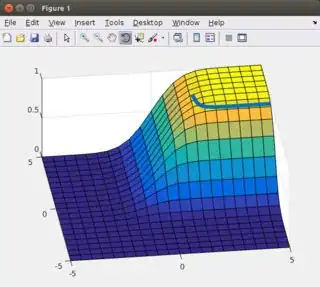
You can use a numerical solver to find the contour as follows:

% plot the distribution
figure;
x = (-5:0.5:5)';
y = (-5:0.5:5)';
[X1,X2] = meshgrid(x',y');
X = [X1(:) X2(:)];
p = mvncdf(X,mu,Sigma);
X3 = reshape(p,length(x),length(y));
surf(X1,X2,X3);

x = (-5:0.1:5)'; % define the x samples at which the contour should be calculated
y0 = zeros(size(x)); % initial guess
y = fsolve(@(y) mvncdf([x y], mu, Sigma) - 0.95, y0); % solve your problem
z = mvncdf([x y],mu,Sigma); % calculate the correspond cdf values
hold on
plot3(x(z>0.94), y(z>0.94), z(z>0.94), 'LineWidth', 5); % plot only the valid solutions, i.e. a solution does not exist for all sample points of x.

enter image description here

To obtain a better numerical representation of the desired contour, you can repeat the above approach for chosen y values. So, your line will better fill the whole graph.

As an alternative, one may use contour to calculate the points on the contour as follows:

figure
[c, h] = contour(X1, X2, X3, [0.95 0.95]);
c(3, :) = mvncdf(c',mu,Sigma);

figure(1)
plot3(c(1, :)', c(2, :)', c(3, :)', 'LineWidth', 5);
xlim([-5 5])
ylim([-5 5])

enter image description here

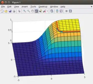
A disadvantage of this approach is that you do not have control over the coarseness of the sampled contour. Secondly, this method uses (interpolation of) the 3D cdf, which is less accurate than the values calculated with fsolve.

m7913d
  • 10,244
  • 7
  • 28
  • 56