How to determine the uncertainty of fit parameters with Python?

Question

I have the following data for x and y:

x   y
1.71    0.0
1.76    5.0
1.81    10.0
1.86    15.0
1.93    20.0
2.01    25.0
2.09    30.0
2.20    35.0
2.32    40.0
2.47    45.0
2.65    50.0
2.87    55.0
3.16    60.0
3.53    65.0
4.02    70.0
4.69    75.0
5.64    80.0
7.07    85.0
9.35    90.0
13.34   95.0
21.43   100.0

For the above data, I am trying to fit the data in the form:

formula

However, there are certain uncertainties associated with x and y, where x has uncertainty of 50% of x and y has a fixed uncertainty. I am trying to determine the uncertainty in the fit parameters with this uncertainties package. But, I am having issues with curve fitting with scipy optimize's curve fit function. I get the following error:

minpack.error: Result from function call is not a proper array of floats.

How do I fix the following error and determine the uncertainty of the fit parameters (a,b and n)?

MWE

from __future__ import division
import numpy as np
import re
from scipy import optimize, interpolate, spatial
from scipy.interpolate import UnivariateSpline
from uncertainties import unumpy


def linear_fit(x, a, b):
    return a * x + b


uncertainty = 0.5
y_error = 1.2
x = np.array([1.71, 1.76, 1.81, 1.86, 1.93, 2.01, 2.09, 2.20, 2.32, 2.47, 2.65, 2.87, 3.16, 3.53, 4.02, 4.69, 5.64, 7.07, 9.35, 13.34, 21.43])
x_uncertainty = x * uncertainty
x = unumpy.uarray(x, x_uncertainty)
y = np.array([0.0, 5.0, 10.0, 15.0, 20.0, 25.0, 30.0, 35.0, 40.0, 45.0, 50.0, 55.0, 60.0, 65.0, 70.0, 75.0, 80.0, 85.0, 90.0, 95.0, 100.0])
y = unumpy.uarray(y, y_error)


n = np.arange(0, 5, 0.005)
coefficient_determination_on = np.empty(shape = (len(n),))
for j in range(len(n)):
    n_correlation = n[j]
    x_fit = 1 / ((x) ** n_correlation)
    y_fit = y
    fit_a_raw, fit_b_raw = optimize.curve_fit(linear_fit, x_fit, y_fit)[0]
    x_prediction = (fit_a_raw / ((x) ** n_correlation)) + fit_b_raw
    y_residual_squares = np.sum((x_prediction - y) ** 2)
    y_total_squares = np.sum((y - np.mean(y)) ** 2)
    coefficient_determination_on[j] = 1 - (y_residual_squares / y_total_squares)

I would assume the `scipy`'s `optimize.curve_fit` method is not implemented to accept `unumpy` arrays. For this type of fitting you might be better off using `scikit-learn` and doing a [Gaussian Process Regression](http://scikit-learn.org/stable/modules/gaussian_process.html) with a combination of exponentiated dot-product (for the actual regression) and white noise (for the uncertainty) kernels. I'm not an expert- try it out and if you have problems pop a question with a `scikit-learn` flag. — Daniel F, Jul 11 '17 at 06:20
Looking through the docs (neat package!) you may be able to use [`uncertainties.wrap`](http://pythonhosted.org/uncertainties/user_guide.html#making-custom-functions-accept-numbers-with-uncertainties) work with `optimize.curve_fit` but that seems like it would take a miracle. Changing my local environment at work is a hell I'm not going to go through for this question to test it though. — Daniel F, Jul 11 '17 at 06:30
`uncertainties` seems to have both derivative and matrix inverse functions, so implementing your own [nonlinear regression](https://en.wikipedia.org/wiki/Non-linear_least_squares) algorithm should be possible. It won't be as fast as `scikit`, but it should work. — Daniel F, Jul 11 '17 at 07:43
@DanielF Not sure if I get it right, but does the Gaussian Process allow for additional errors in `x` or only in `y`? If yes, where is it set? — mikuszefski, Jul 11 '17 at 14:20
Are you sure about the 50% on x? The fact that with this small steps it is monotonic contradicts this a bit. Note the values at y approc 25 could be basically anything between 1 and 3 and yet you have a neat increase of about 5% to 10%. With a 50% error this monotonic behaviour should be lost in noise. — mikuszefski, Jul 18 '17 at 06:34
Note for your data you'd have `x= a*y**n+b` not `y= a*x**n+b`. In the latter one you do not have a proper intercept. and it really looks to be of type `(x-x0)**(1/n)` BTW is `n` supposed to be an integer or if you look at it the other way round an integer root? — mikuszefski, Jul 19 '17 at 09:56

score 4 · Answer 1 · answered Jul 18 '17 at 14:54

Let me first preface this with this problem being impossible to solve "nicely" given that you want to solve for a, b and n. This is because for a fixed n, your problem admits a closed form solution, while if you let n be free, it does not, and in fact the problem may have multiple solutions. Hence classical error analysis (such as that used by uncertanities) breaks down and you have to resort to other methods.

The case `n` fixed

If n is fixed, your problem is that the libraries you call do not support uarray, so you have to make a workaround. Thankfully, linear fitting (under the l2-distance) is simply Linear least squares which admits a closed form solution, requiring only padding the values with ones and then solving the normal equations.

Where:

You could do it like this:

import numpy as np
from uncertainties import unumpy

uncertainty = 0.5
y_error = 1.2
n = 1.0

# Define x and y
x = np.array([1.71, 1.76, 1.81, 1.86, 1.93, 2.01, 2.09, 2.20, 2.32, 2.47, 2.65,
              2.87, 3.16, 3.53, 4.02, 4.69, 5.64, 7.07, 9.35, 13.34, 21.43])
# Take power of x values according to n
x_pow = x ** n
x_uncertainty = x_pow * uncertainty
x_fit = unumpy.uarray(np.c_[x_pow, np.ones_like(x)],
                      np.c_[x_uncertainty, np.zeros_like(x_uncertainty)])

y = np.array([0.0, 5.0, 10.0, 15.0, 20.0, 25.0, 30.0, 35.0, 40.0, 45.0, 50.0,
              55.0, 60.0, 65.0, 70.0, 75.0, 80.0, 85.0, 90.0, 95.0, 100.0])
y_fit = unumpy.uarray(y, y_error)

# Use normal equations to find coefficients
inv_mat = unumpy.ulinalg.pinv(x_fit.T.dot(x_fit))
fit_a, fit_b = inv_mat.dot(x_fit.T.dot(y_fit))

print('fit_a={}, fit_b={}'.format(fit_a, fit_b))

Result:

fit_a=4.8+/-2.6, fit_b=28+/-10

The case `n` unknown

With n unknown, you really are in some trouble since the problem is non-convex. Here, linear error analysis (as performed by uncertainties) will not work.

One solution is to perform Bayesian inference, using some package like pymc. If you are interested in this, I could try to make a writeup, but it would not be as clean as above.

Concerning lack of `uarray` support [uncertanties.wrap()](https://github.com/lebigot/uncertainties/blob/2d963e923bb4e622d720621255bd206af7043947/uncertainties/core.py#L436-L549) might do the trick. Even better, there's direct `numpy` support via [`unumpy`](https://uncertainties-python-package.readthedocs.io/en/latest/numpy_guide.html) — Tobias Kienzler, Mar 19 '21 at 09:29
(I see OP already uses `uarray`, and `wrap` was [mentioned](https://stackoverflow.com/questions/45026332/how-to-determine-the-uncertainty-of-fit-parameters-with-python#comment77027865_45026332) as well, though not further pursued by anyone, it seems) — Tobias Kienzler, Mar 19 '21 at 09:41

mikuszefski · Answer 2 · 2017-07-21T08:58:13.607

Following a little the case of a linear function I think it might be done similar. Solving for the Lagrangian, though, seems to be very tedious, while possible of course. A made up a different measure that seems plausible and should give very similar result. Taking the error ellipse I rescale it such that the graph becomes a tangent. I take the distance to that touching point (X_k,Y_k) as measure for chi-square, which is calculated from (x_k-X_k/sx_k)**2+(y_k-Y_k/sy_k)**2. It is plausible as in case of pure y-errors this is the standard least square fit. For pure x-errors it just switches. For equal x,y-errors it would give the perpendicular rule, i.e. shortest distance. With the according chi-square function scipy.optimize.leastsq already provides the covariance matrix approximated from the Hesse. In detail one has to scale it, though. 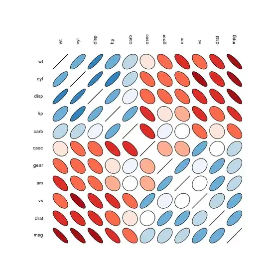Also note that the parameters are strongly correlated.

My procedure looks as follows:

import matplotlib
matplotlib.use('Qt5Agg')

import matplotlib.pyplot as plt
import numpy as np
import myModules.multipoleMoments as mm 
from random import random
from scipy.optimize import minimize,leastsq


###for gaussion distributed errors
def boxmuller(x0,sigma):
    u1=random()
    u2=random()
    ll=np.sqrt(-2*np.log(u1))
    z0=ll*np.cos(2*np.pi*u2)
    z1=ll*np.cos(2*np.pi*u2)
    return sigma*z0+x0, sigma*z1+x0


###function to fit
def f(t,c,d,n):
    return c+d*np.abs(t)**n


###to create some test data
def test_data(c,d,n, xList,const_sx,rel_sx,const_sy,rel_sy):
    yList=[f(t,c,d,n) for t in xList]
    xErrList=[ boxmuller(x,const_sx+x*rel_sx)[0] for x in xList]
    yErrList=[ boxmuller(y,const_sy+y*rel_sy)[0] for y in yList]
    return xErrList,yErrList


###how to rescale the ellipse to make fitfunction a tangent
def elliptic_rescale(x,c,d,n,x0,y0,sa,sb):
    y=f(x,c,d,n)
    r=np.sqrt((x-x0)**2+(y-y0)**2)
    kappa=float(sa)/float(sb)
    tau=np.arctan2(y-y0,x-x0)
    new_a=r*np.sqrt(np.cos(tau)**2+(kappa*np.sin(tau))**2)
    return new_a


###for plotting ellipses
def ell_data(a,b,x0=0,y0=0):
    tList=np.linspace(0,2*np.pi,150)
    k=float(a)/float(b)
    rList=[a/np.sqrt((np.cos(t))**2+(k*np.sin(t))**2) for t in tList]
    xyList=np.array([[x0+r*np.cos(t),y0+r*np.sin(t)] for t,r in zip(tList,rList)])
    return xyList


###residual function to calculate chi-square
def residuals(parameters,dataPoint):#data point is (x,y,sx,sy)
    c,d,n= parameters
    theData=np.array(dataPoint)
    best_t_List=[]
    for i in range(len(dataPoint)):
        x,y,sx,sy=dataPoint[i][0],dataPoint[i][1],dataPoint[i][2],dataPoint[i][3]
        ###getthe point on the graph where it is tangent to an error-ellipse
        ed_fit=minimize(elliptic_rescale,0,args=(c,d,n,x,y,sx,sy) )
        best_t=ed_fit['x'][0]
        best_t_List+=[best_t]
    best_y_List=[f(t,c,d,n) for t in best_t_List]
    ##weighted distance not squared yet, as this is done by scipy.optimize.leastsq
    wighted_dx_List=[(x_b-x_f)/sx for x_b,x_f,sx in zip( best_t_List,theData[:,0], theData[:,2] ) ]
    wighted_dy_List=[(x_b-x_f)/sx for x_b,x_f,sx in zip( best_y_List,theData[:,1], theData[:,3] ) ]
    return wighted_dx_List+wighted_dy_List


###some start values
cc,dd,nn=2.177,.735,1.75
ssaa,ssbb=1,3
xx0,yy0=2,3
csx,rsx=.1,.05
csy,rsy=.4,.00

####some data
xThData=np.linspace(0,3,15)
yThData=[ f(t, cc,dd,nn) for t in xThData]

###some noisy data
xNoiseData,yNoiseData=test_data(cc,dd,nn, xThData, csx,rsx, csy,rsy)
xGuessdError=[csx+rsx*x for x in xNoiseData]
yGuessdError=[csy+rsy*y for y in yNoiseData]

###plot that
fig1 = plt.figure(1)
ax=fig1.add_subplot(1,1,1)
ax.plot(xThData,yThData)
ax.errorbar(xNoiseData,yNoiseData, xerr=xGuessdError, yerr=yGuessdError, fmt='none',ecolor='r')

#### and plot...
for i in range(len(xNoiseData)):
    ###...an elliple on the error values
    el0=ell_data(xGuessdError[i],yGuessdError[i],x0=xNoiseData[i],y0=yNoiseData[i])
    ax.plot(*zip(*el0),linewidth=1, color="#808080",linestyle='-')
    ####...as well as a scaled version that touches the original graph. This gives the error shortest distance to that graph
    ed_fit=minimize(elliptic_rescale,0,args=(cc,dd,nn,xNoiseData[i],yNoiseData[i],xGuessdError[i],yGuessdError[i]) )
    best_t=ed_fit['x'][0]
    best_a=elliptic_rescale(best_t,cc,dd,nn,xNoiseData[i],yNoiseData[i],xGuessdError[i],yGuessdError[i])
    el0=ell_data(best_a,best_a/xGuessdError[i]*yGuessdError[i],x0=xNoiseData[i],y0=yNoiseData[i])
    ax.plot(*zip(*el0),linewidth=1, color="#a000a0",linestyle='-')

###Now fitting
zipData=zip(xNoiseData,yNoiseData, xGuessdError, yGuessdError)    
estimate = [2.0,1,2.5]
bestFitValues, cov,info,mesg, ier = leastsq(residuals, estimate,args=(zipData), full_output=1)
print bestFitValues
####covariance matrix
####note e.g.: https://stackoverflow.com/questions/14854339/in-scipy-how-and-why-does-curve-fit-calculate-the-covariance-of-the-parameter-es
s_sq = (np.array(residuals(bestFitValues, zipData))**2).sum()/(len(zipData)-len(estimate))
pcov = cov * s_sq
print pcov



#### and plot the result...
ax.plot(xThData,[f(x,*bestFitValues) for x in xThData])
for i in range(len(xNoiseData)):
    ####...as well as a scaled ellipses that touches the fitted graph. 
    ed_fit=minimize(elliptic_rescale,0,args=(bestFitValues[0],bestFitValues[1],bestFitValues[2],xNoiseData[i],yNoiseData[i],xGuessdError[i],yGuessdError[i]) )
    best_t=ed_fit['x'][0]
    best_a=elliptic_rescale(best_t,bestFitValues[0],bestFitValues[1],bestFitValues[2],xNoiseData[i],yNoiseData[i],xGuessdError[i],yGuessdError[i])
    el0=ell_data(best_a,best_a/xGuessdError[i]*yGuessdError[i],x0=xNoiseData[i],y0=yNoiseData[i])
    ax.plot(*zip(*el0),linewidth=1, color="#f0a000",linestyle='-')

#~ ax.grid(None)
plt.show()

The blue graph is the original function. The data points with red error bars are calculated from this. A grey ellipse shows the "line of constant probability density". Purple ellipses have the original graph as tangent, orange ellipses have the fit as tangent

Here best fit values are (not your data!):

[ 2.16146783  0.80204967  1.69951865]

Covariance matrix has the form:

[[ 0.0644794  -0.05418743  0.05454876]
 [-0.05418743  0.07228771 -0.08172885]
 [ 0.05454876 -0.08172885  0.10173394]]

Edit Thinking about the "elliptic distance" I believe that this is exactly what the Lagrangian approach in the linked paper does. Only that for a straight line you can write down an exact solution while in this case you cannot.

Update I had some problems with the OP's data. It works with rescaling, though. As slope and exponent are highly correlated, I first had to figure out how the covariance matrix changes for rescaled data. Details can be found in J. Phys. Chem. 105 (2001) 3917

Using the function definitions from above the data treatment would look like:

###some start values
cc,dd,nn=.2,1,7.5
csx,rsx=2.0,.0
csy,rsy=0,.5

###some noisy data
yNoiseData=np.array([1.71,1.76, 1.81, 1.86, 1.93, 2.01, 2.09, 2.20, 2.32, 2.47, 2.65, 2.87, 3.16, 3.53, 4.02, 4.69, 5.64, 7.07, 9.35,13.34,21.43])
xNoiseData=np.array([0.0,5.0,10.0,15.0,20.0,25.0,30.0,35.0,40.0,45.0,50.0,55.0,60.0,65.0,70.0,75.0,80.0,85.0,90.0,95.0,100.0])

xGuessdError=[csx+rsx*x for x in xNoiseData]
yGuessdError=[csy+rsy*y for y in yNoiseData]

###plot that
fig1 = plt.figure(1)
ax=fig1.add_subplot(1,2,2)
bx=fig1.add_subplot(1,2,1)
ax.errorbar(xNoiseData,yNoiseData, xerr=xGuessdError, yerr=yGuessdError, fmt='none',ecolor='r')

####rescaling        

print "\n++++++++++++++++++++++++  scaled ++++++++++++++++++++++++\n"
alpha=.05
beta=.01
xNoiseDataS   = [   beta*x for x in   xNoiseData   ]
yNoiseDataS   = [   alpha*x for x in   yNoiseData   ]
xGuessdErrorS  = [   beta*x for x in   xGuessdError ]
yGuessdErrorS  = [   alpha*x for x in   yGuessdError ] 


xtmp=np.linspace(0,1.1,25)
bx.errorbar(xNoiseDataS,yNoiseDataS, xerr=xGuessdErrorS, yerr=yGuessdErrorS, fmt='none',ecolor='r')


###Now fitting
zipData=zip(xNoiseDataS,yNoiseDataS, xGuessdErrorS, yGuessdErrorS)
estimate = [.1,1,7.5]
bestFitValues, cov,info,mesg, ier = leastsq(residuals, estimate,args=(zipData), full_output=1)
print bestFitValues
plt.plot(xtmp,[ f(x,*bestFitValues)for x in xtmp])
####covariance matrix
s_sq = (np.array(residuals(bestFitValues, zipData))**2).sum()/(len(zipData)-len(estimate))
pcov = cov * s_sq
print pcov

#### scale back  
print "\n++++++++++++++++++++++++  scaled back ++++++++++++++++++++++++\n"


realBestFitValues= [bestFitValues[0]/alpha, bestFitValues[1]/alpha*(beta)**bestFitValues[2],bestFitValues[2] ]
print realBestFitValues
uMX = np.array( [[1/alpha,0,0],[0,beta**bestFitValues[2]/alpha,bestFitValues[1]/alpha*beta**bestFitValues[2]*np.log(beta)],[0,0,1]] )
uMX_T = uMX.transpose()
realCov = np.dot(uMX, np.dot(pcov,uMX_T))
print realCov

for i,para in enumerate(["b","a","n"]):
    print para+" = "+"{:.2e}".format(realBestFitValues[i])+" +/- "+"{:.2e}".format(np.sqrt(realCov[i,i]))

ax.plot(xNoiseData,[f(x,*realBestFitValues) for x in xNoiseData])

plt.show()

So the data is reasonably fitted. I think, however, there is a linear term as well.

The output provides:

++++++++++++++++++++++++  scaled ++++++++++++++++++++++++

[ 0.09788886  0.69614911  5.2221032 ]
[[  1.25914194e-05   2.86541696e-05   6.03957467e-04]
 [  2.86541696e-05   3.88675025e-03   2.00199108e-02]
 [  6.03957467e-04   2.00199108e-02   1.75756532e-01]]

++++++++++++++++++++++++  scaled back ++++++++++++++++++++++++

[1.9577772055183396, 5.0064036934715239e-10, 5.2221031993990517]
[[  5.03656777e-03  -2.74367539e-11   1.20791493e-02]
 [ -2.74367539e-11   8.69854174e-19  -3.90815222e-10]
 [  1.20791493e-02  -3.90815222e-10   1.75756532e-01]]

b = 1.96e+00 +/- 7.10e-02
a = 5.01e-10 +/- 9.33e-10
n = 5.22e+00 +/- 4.19e-01

One can see strong correlation of slope and exponent in the covariance matrix. Also note that the error of the slope is huge.

BTW Using as model b+a*x**n + e*x I get

++++++++++++++++++++++++  scaled ++++++++++++++++++++++++

[ 0.08050174  0.78438855  8.11845402  0.09581568]
[[  5.96210962e-06   3.07651631e-08  -3.57876577e-04  -1.75228231e-05]
 [  3.07651631e-08   1.39368435e-03   9.85025139e-03   1.83780053e-05]
 [ -3.57876577e-04   9.85025139e-03   1.85226736e-01   2.26973118e-03]
 [ -1.75228231e-05   1.83780053e-05   2.26973118e-03   7.92853339e-05]]

++++++++++++++++++++++++  scaled back ++++++++++++++++++++++++

[1.6100348667765145, 9.0918698097511416e-16, 8.1184540175879985, 0.019163135651422442]
[[  2.38484385e-03   2.99690170e-17  -7.15753154e-03  -7.00912926e-05]
 [  2.99690170e-17   3.15340690e-30  -7.64119623e-16  -1.89639468e-18]
 [ -7.15753154e-03  -7.64119623e-16   1.85226736e-01   4.53946235e-04]
 [ -7.00912926e-05  -1.89639468e-18   4.53946235e-04   3.17141336e-06]]
b = 1.61e+00 +/- 4.88e-02
a = 9.09e-16 +/- 1.78e-15
n = 8.12e+00 +/- 4.30e-01
e = 1.92e-02 +/- 1.78e-03

Sure, fits always get better if you add parameters, but I think this looks sort of reasonable here (it might even be that it is b + a*x**n+e*x**m, but this is leading too far.)

How to determine the uncertainty of fit parameters with Python?

2 Answers2

The case `n` fixed

The case `n` unknown

Linked

How to determine the uncertainty of fit parameters with Python?

2 Answers2

The case n fixed

The case n unknown

Linked

The case `n` fixed

The case `n` unknown