0

So i have the template layout in the picture attached below. I would like to know how to link the Spin button to able to show month by month when i click on the spin button. Here is the formula i have so far, everything working fine except for the chart doesn't connect to the spin.

E4 formula : ="Monthly "&E5&" - Audit Sheet Delivery"
data for eat month for LATE row:=IFERROR(VLOOKUP(G3,$A$4:$C$6000,2,FALSE)," ")
Same for On-Time:=IFERROR(VLOOKUP(G3,$A$4:$C$6000,3,FALSE)," ")
Spin button link to cell $E$5

I have created define name for each Month, Late and On-Time and linked it to the chart but it doesn't work. Please point out what i have to do in this case. Also, please show the code on here due to i am new to this. Thanksenter image description here

enter image description here

Patrick Trentin
  • 7,126
  • 3
  • 23
  • 40
Ryan Nguyen
  • 25
  • 1
  • 9
  • 1
    So what do you want to happen when you click up or down on the spin button? – dwirony Jun 06 '18 at 18:41
  • Not sure if useful but have you considered a timeline slicer? – QHarr Jun 06 '18 at 18:57
  • When i click up and down spin button, the Title of the chart change accordingly to cell E4 but the chart stay the same.I just wonder how can i link the spin button with the chart so it will change data on the chart. – Ryan Nguyen Jun 06 '18 at 20:41
  • QHarr-I know how to use the slicer but i want to keep it clean and use only spin button or scroll button. It will look better – Ryan Nguyen Jun 06 '18 at 20:42
  • I guess linked cell can index into months for plotting – QHarr Jun 06 '18 at 21:32
  • And, as @dwirony points out, what change should we see when you press the spin button? A visual image of the desired result would help. – QHarr Jun 07 '18 at 04:19

3 Answers3

0

How to do anything anything Excel can do, but with VBA code:

Virtually anything you can do manually in Excel (ie, via the ribbons/toolbars) has an equivalent in VBA.

If you are unsure of which VBA method or property to use, you can turn on the macro recorder and manually perform the action. The macro recorder translates your actions into Visual Basic code. After you record your actions, you can modify the code to do exactly what you want.

There are some limitations to recording macros, so if needed, certain actions have to be added after recording, such as conditional branches (eg., IF statements), variables usage loops, error handling, and text selections made with the mouse (however keyboard combinations do record).


Record an action:

For example, if you want to automate the process of saving the file with a new name, but you don't know which property or method to use, you could do this:

  1. On the Developer ribbon, click img
    Change the default macro name to a name of your choice and click OK to start the recorder.
  2. Hit F12 to open the Save As... dialog and save the file with a new name.
  3. On the Developer ribbon, click img
  4. On the Developer ribbon, click img Macros.
  5. Select the macro name that you assigned (in Step 2) and click Edit to view the VBA code within.

See the tips & resources at the links below to help get you started with automatizing Excel (and other Office applications) using VBA code.


More information:


Original Post:

How to filter a chart

The ability to filter a chart by month is built-in to Excel. After you create a chart, you can change the data series in two ways:

  • Use chart filters to show or hide data in your chart, or,

  • Use the Select Data Source dialog box to edit the data in your series or rearrange them on your chart.

Filter data in your chart

  1. Click anywhere in your chart.

  2. Click the Chart Filters button Chart Filters button next to the chart.

  3. On the Values tab, check or uncheck the series or categories you want to show or hide. Values tab in the Chart Filters gallery

  4. Click Apply.

  5. If you want to edit or rearrange the data in your series, click Select Data, and then follow steps 2-4 in the next section.

Once you know how to use the filters, you can record a macro while filtering as required, an use the code for buttons or other controls.


More Information:

ashleedawg
  • 20,365
  • 9
  • 72
  • 105
  • Month by month made me think timeline slicer as an additional option. – QHarr Jun 06 '18 at 19:25
  • Yeah, i did use the splicer before. but it took too much space. I know there is away you can use either spin button or scroll button with formula to change the data on the chart by clicking on the arrow up and down. it is better and the title change accordingly to the data. – Ryan Nguyen Jun 06 '18 at 20:56
  • It's a *slicer* and it doesn't have to remain visible. Yes of course there's "a way"... in fact there are several ways it could work; the issue is finding the one right for your data and your experience level. – ashleedawg Jun 07 '18 at 02:08
  • @RyanNguyen You didn't mention any issue with my answer. You could just use the chart filters, programmatically controlled bu your buttons. Problem solved? – ashleedawg Jun 07 '18 at 02:08
  • ashleedawg. How you link up the chart filter with the spin button? i would love to know how. – Ryan Nguyen Jun 07 '18 at 14:58
  • @RyanNguyen I added more information to my answer to help get you started. – ashleedawg Jun 08 '18 at 00:22
0

Thanks you all for your help. I did figure out one way to make it work for me. However, i will more than happy to learn new way or a better way to use spin button and scroll button to changing my chart.

  1. Changes data layout table
  2. Using index formula and vlookup (Cell F19, G19,H19) formula included in picture below)
  3. Changes define name formula to pull data from Cell (Cell F19, G19,H19).
  4. Now i can click on my spin button and the chart changing month by month for me.

It is working fine for me. But i love to learn more if anyone can show me a better way to do it. Please include pictures and formula in your answer. It will help me and other easy to follow it. Thanksenter image description here

Ryan Nguyen
  • 25
  • 1
  • 9
0

Steps

This is broadly similar to yours. Below is just meant to show you how to use dynamic named ranges as chart series sources. If you later decide to specify start and end ranges of months, you could use this same model and have the start and end indexes generate the height argument for Offset thus being able to plot ranges (though they would be aggregate).

Using the same data layout as in your answer.


① Add a forms control spin button, assign its linked cell as K3, then put the font to white so it is not visible. Its values run from 1-12 with increment 1.


② I then create two dynamic ranges:

  1. LATE with formula =OFFSET(Sheet1!$G$4,Sheet1!$K$3-1,0,1,1)
  2. OnTime with formula =OFFSET(Sheet1!$H$4,Sheet1!$K$3-1,0,1,1)

You can add these via name manager (Alt+F3)

Name manager:

Name manager


③ I then insert a bar chart and add two series which use these dynamic named ranges as their source:
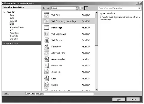
Late series for chart

The above is for Late and this is repeated for OnTime. Note that the workbook name goes before the reference to the dynamic range.


④ In J2 I enter the chart title text "Monthly - 5 KPI Delivery" and point the chart title at this with = J2 in formula bar whilst chart title is selected on the chart.


K2 has the formula =INDEX(F4:F15,K3) and is used to retrieve the Month name from the list of months via Index with row argument the linked cell value from the spin button.

I then edit the chart X axis source with formula =Sheet1!$K$2 so the month name appears on the bottom of the chart.


⑥ Finally, any other chart sprucing you like. I chose to group and lock the chart and spin button together so they will move as a unit and to ensure data point values where shown.


Final result:
Output


In action:

Test run

X axis

QHarr
  • 83,427
  • 12
  • 54
  • 101