Detecting seasonality without two full periods of data

Question

I have the following dataset (df) with 20 months:

There should be seasonality, and I want to estimate this and remove it. I attempted this using the below code:

df <- ts(df$price, frequency = 12, start = c(2016,8))
decompose_df <- decompose( , "additive")
adjust_df<- df- decompose_df $seasonal
plot(adjust_df)

But as I only have 20 months and not two full periods of data, I get the below error:

Error in decompose(df, "additive") : 
time series has no or less than 2 periods

Is there a way I can test and remove this seasonality? Even though I only have 20 periods when I need 24.

You can't, unless you specify a sub-annual frequency.The intuition of why you can't is simple: if you only have enough data to see one full cycle (meaning you can't see the pattern repeat even once), how would you know that is a seasonal effect and not just an anomaly? Check this answer for more explanation: https://stackoverflow.com/questions/12330581/too-few-periods-for-decompose — acylam, Jul 13 '18 at 17:07
Thanks. The data is to do with house prices and just from general research and intuition I know it is seasonal, so I want to remove it. So if I want to overcome this and get some estimate, I use a sub-annual frequency? How would I choose this frequency given I have 20 observations? And how would I do this and then remove the seasonality? — PMc, Jul 13 '18 at 17:19

score 12 · Accepted Answer · answered Jul 14 '18 at 00:05

It's not possible using the usual methods of decomposition because they estimate seasonality using at least as many degrees of freedom as there are seasonal periods. As @useR has pointed out, you need at least two observations per seasonal period to be able to distinguish seasonality from noise.

However, if you are willing to assume that the seasonality is relatively smooth, then you can estimate it using fewer degrees of freedom. For example, you can approximate the seasonal pattern using Fourier terms with a few parameters.

df <- ts(c(
2735.869,2857.105,2725.971,2734.809,2761.314,2828.224,2830.284,2758.149,
2774.943,2782.801,2861.970,2878.688,3049.229,3029.340,3099.041,3071.151,
3075.576,3146.372,3005.671,3149.381), start=c(2016,8), frequency=12)

library(forecast)
library(ggplot2)
decompose_df <- tslm(df ~ trend + fourier(df, 2))
trend <- coef(decompose_df)[1] + coef(decompose_df)['trend']*seq_along(df)
components <- cbind(
  data = df,
  trend = trend,  
  season = df - trend - residuals(decompose_df),
  remainder = residuals(decompose_df)
)
autoplot(components, facet=TRUE)

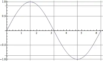
You can adjust the order of the Fourier terms as required. I've used 2 here. For monthly data, the maximum you can use is 6, but that will give a model with 13 degrees of freedom which is way too many with only 20 observations. If you don't know about Fourier terms for seasonality, see https://otexts.org/fpp2/useful-predictors.html#fourier-series.

Now we can remove the seasonal component to get the seasonally adjusted data.

adjust_df <- df - components[,'season']
autoplot(df, series="Data") + autolayer(adjust_df, series="Seasonally adjusted")

Brilliant thank you for that. Just one question. I too used 2 Fourier terms, although I tested this for up to and including 6 terms. **How do you know which is the most appropriate number of terms?** I used `summary(decompose_jily_psqm)` and looked at the p-values. And only `S1-12` and `S2-12` were significant, hence why I picked 2 terms. However, `C1-12` and `C2-12` were never significant, although I am not aware if this is important or not. — PMc, Jul 14 '18 at 09:25
An extended version of this answer is at https://robjhyndman.com/hyndsight/tslm-decomposition/. You minimize AICc or CV, as explained there. Also significance is not really important here. — Rob Hyndman, Jul 17 '18 at 05:44

Detecting seasonality without two full periods of data

1 Answers1