Fastest code to calculate distance between points in 2D numpy array with cyclic (periodic) boundary conditions

Question

I know how to calculate the Euclidean distance between points in an array using scipy.spatial.distance.cdist

Similar to answers to this question: Calculate Distances Between One Point in Matrix From All Other Points

However, I would like to make the calculation assuming cyclic boundary conditions, e.g. so that point [0,0] is distance 1 from point [0,n-1] in this case, not a distance of n-1. (I will then make a mask for all points within a threshold distance of my target cells, but that is not central to the question).

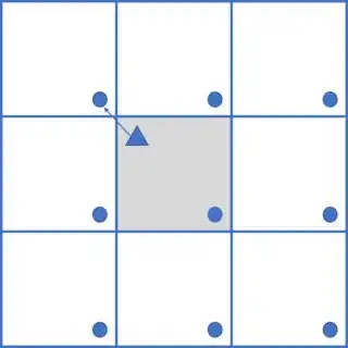
The only way I can think of is to repeat the calculation 9 times, with the domain indices having n added/subtracted in the x, y and then x&y directions, and then stacking the results and finding the minimum across the 9 slices. To illustrate the need for 9 repetitions, I put together a simple schematic with just 1 J-point, marked with a circle, and which shows an example where the cell marked by the triangle in this case has its nearest neighbour in the domain reflected to the top-left.

this is the code I developed for this using cdist:

import numpy as np
from scipy import spatial
    
n=5 # size of 2D box (n X n points)
np.random.seed(1) # to make reproducible
a=np.random.uniform(size=(n,n)) 
i=np.argwhere(a>-1)  # all points, for each loc we want distance to nearest J 
j=np.argwhere(a>0.85) # set of J locations to find distance to.

# this will be used in the KDtree soln 
global maxdist
maxdist=2.0

def dist_v1(i,j):
    dist=[]
    # 3x3 search required for periodic boundaries.
    for xoff in [-n,0,n]:
        for yoff in [-n,0,n]:
            jo=j.copy()
            jo[:,0]-=xoff
            jo[:,1]-=yoff
            dist.append(np.amin(spatial.distance.cdist(i,jo,metric='euclidean'),1)) 
    dist=np.amin(np.stack(dist),0).reshape([n,n])
    return(dist)

This works, and produces e.g. :

print(dist_v1(i,j))


[[1.41421356 1.         1.41421356 1.41421356 1.        ]
 [2.23606798 2.         1.41421356 1.         1.41421356]
 [2.         2.         1.         0.         1.        ]
 [1.41421356 1.         1.41421356 1.         1.        ]
 [1.         0.         1.         1.         0.        ]]

The zeros obviously mark the J points, and the distances are correct (this EDIT corrects my earlier attempts which was incorrect).

Note that if you change the last two lines to stack the raw distances and then only use one minimum like this :

def dist_v2(i,j):
    dist=[]
    # 3x3 search required for periodic boundaries.
    for xoff in [-n,0,n]:
        for yoff in [-n,0,n]:
            jo=j.copy()
            jo[:,0]-=xoff
            jo[:,1]-=yoff
            dist.append(spatial.distance.cdist(i,jo,metric='euclidean')) 
    dist=np.amin(np.dstack(dist),(1,2)).reshape([n,n])
    return(dist)

it is faster for small n (<10) but considerably slower for larger arrays (n>10)

...but either way, it is slow for my large arrays (N=500 and J points number around 70), this search is taking up about 99% of the calculation time, (and it is a bit ugly too using the loops) - is there a better/faster way?

The other options I thought of were:

1. scipy.spatial.KDTree.query_ball_point

With further searching I have found that there is a function scipy.spatial.KDTree.query_ball_point which directly calculates the coordinates within a radius of my J-points, but it doesn't seem to have any facility to use periodic boundaries, so I presume one would still need to somehow use a 3x3 loop, stack and then use amin as I do above, so I'm not sure if this will be any faster.

I coded up a solution using this function WITHOUT worrying about the periodic boundary conditions (i.e. this doesn't answer my question)

def dist_v3(n,j):
    x, y = np.mgrid[0:n, 0:n]
    points = np.c_[x.ravel(), y.ravel()]
    tree=spatial.KDTree(points)
    mask=np.zeros([n,n])
    for results in tree.query_ball_point((j), maxdist):
        mask[points[results][:,0],points[results][:,1]]=1
    return(mask)

Maybe I'm not using it in the most efficient way, but this is already as slow as my cdist-based solutions even without the periodic boundaries. Including the mask function in the two cdist solutions, i.e. replacing the return(dist) with return(np.where(dist<=maxdist,1,0)) in those functions, and then using timeit, I get the following timings for n=100:

from timeit import timeit

print("cdist v1:",timeit(lambda: dist_v1(i,j), number=3)*100)
print("cdist v2:",timeit(lambda: dist_v2(i,j), number=3)*100)
print("KDtree:", timeit(lambda: dist_v3(n,j), number=3)*100)

cdist v1: 181.80927299981704
cdist v2: 554.8205785999016
KDtree: 605.119637199823

2. Make an array of relative coordinates for points within a set distance of [0,0] and then manually loop over the J points setting up a mask with this list of relative points - This has the advantage that the "relative distance" calculation is only performed once (my J points change each timestep), but I suspect the looping will be very slow.

3. Precalculate a set of masks for EVERY point in the 2D domain, so in each timestep of the model integration I just pick out the mask for the J-point and apply. This would use a LOT of memory (proportional to n^4) and perhaps is still slow as you need to loop over J points to combine the masks.

Answer 1

I'll show an alternative approach from an image processing perspective, which may be of interest to you, regardless of whether it's the fastest or not. For convenience, I've only implemented it for an odd n.

Rather than considering a set of nxn points i, let's instead take the nxn box. We can consider this as a binary image. Let each point in j be a positive pixel in this image. For n=5 this would look something like:

Now let's think about another concept from image processing: Dilation. For any input pixel, if it has a positive pixel in its neighborhood, the output pixel will be 1. This neighborhood is defined by what is called the Structuring Element: a boolean kernel where the ones will show which neighbors to consider.

Here's how I define the SE for this problem:

Y, X = np.ogrid[-n:n+1, -n:n+1]
SQ = X*X+Y*Y

H = SQ == r

Intuitively, H is a mask denoting 'all points from the center at who satisfy the equation x*x+y*y=r. That is, all points in H lie at sqrt(r) distance from the center. Another visualization and it'll be absolutely clear:

It is an ever expanding pixel circle. Each white pixel in each mask denotes a point where the distance from the center pixel is exactly sqrt(r). You might also be able to tell that if we iteratively increase the value of r, we're actually steadily covering all the pixel locations around a particular location, eventually covering the entire image. (Some values of r don't give responses, because no such distance sqrt(r) exists for any pair of points. We skip those r values - like 3.)

So here's what the main algorithm does.

• We will incrementally increase the value of r starting from 0 to some high upper limit.
• At each step, if any position (x,y) in the image gives a response to dilation, that means that there is a j point at exactly sqrt(r) distance from it!
• We can find a match multiple times; we'll only keep the first match and discard further matches for points. We do this till all pixels (x,y) have found their minimum distance / first match.

So you could say that this algorithm is dependent on the number of unique distance pairs in the nxn image.

This also implies that if you have more and more points in j, the algorithm will actually get faster, which goes against common sense!

The worst case for this dilation algorithm is when you have the minimum number of points (exactly one point in j), because then it would need to iterate r to a very high value to get a match from points far away.

In terms of implementing:

n=5 # size of 2D box (n X n points)
np.random.seed(1) # to make reproducible
a=np.random.uniform(size=(n,n)) 
I=np.argwhere(a>-1)  # all points, for each loc we want distance to nearest J 
J=np.argwhere(a>0.85)

Y, X = np.ogrid[-n:n+1, -n:n+1]
SQ = X*X+Y*Y

point_space = np.zeros((n, n))
point_space[J[:,0], J[:,1]] = 1


C1 = point_space[:, :n//2]
C2 = point_space[:, n//2+1:]
C = np.hstack([C2, point_space, C1])

D1 = point_space[:n//2, :]
D2 = point_space[n//2+1:, :]
D2_ = np.hstack([point_space[n//2+1:, n//2+1:],D2,point_space[n//2+1:, :n//2]])
D1_ = np.hstack([point_space[:n//2:, n//2+1:],D1,point_space[:n//2, :n//2]])
D = np.vstack([D2_, C, D1_])
p = (3*n-len(D))//2
D = np.pad(D, (p,p), constant_values=(0,0))

plt.imshow(D, cmap='gray')
plt.title(f'n={n}')

If you look at the image for n=5, you can tell what I've done; I've simply padded the image with its four quadrants in a way to represent the cyclic space, and then added some additional zero padding to account for the worst case search boundary.

@nb.jit
def dilation(image, output, kernel, N, i0, i1):
    for i in range(i0,i1):
        for j in range(i0, i1):
            a_0 = i-(N//2)
            a_1 = a_0+N
            b_0 = j-(N//2)
            b_1 = b_0+N
            neighborhood = image[a_0:a_1, b_0:b_1]*kernel
            if np.any(neighborhood):
                output[i-i0,j-i0] = 1
    return output

@nb.njit(cache=True)
def progressive_dilation(point_space, out, total, dist, SQ, n, N_):
    for i in range(N_):
        if not np.any(total): 
            break
            
        H = SQ == i

        rows, cols = np.nonzero(H)
        if len(rows) == 0: continue
        
        rmin, rmax = rows.min(), rows.max()
        cmin, cmax = cols.min(), cols.max()

        H_ = H[rmin:rmax+1, cmin:cmax+1]
        
        out[:] = False 
        out = dilation(point_space, out, H_, len(H_), n, 2*n)
        
        idx = np.logical_and(out, total)
        
        for a, b in  zip(*np.where(idx)):
            dist[a, b] = i
        
        total = total * np.logical_not(out)
    return dist

def dilateWrap(D, SQ, n):
    out = np.zeros((n,n), dtype=bool)
    total = np.ones((n,n), dtype=bool)
    dist=-1*np.ones((n,n))
    dist = progressive_dilation(D, out, total, dist, SQ, n, 2*n*n+1)
    return dist

dout = dilateWrap(D, SQ, n)

If we visualize dout, we can actually get an awesome visual representation of the distances.

The dark spots are basically positions where j points were present. The brightest spots naturally means points farthest away from any j. Note that I've kept the values in squared form to get an integer image. The actual distance is still one square root away. The results match with the outputs of the ball park algorithm.

# after resetting n = 501 and rerunning the first block

N = J.copy()
NE = J.copy()
E = J.copy()
SE = J.copy()
S = J.copy()
SW = J.copy()
W = J.copy()
NW = J.copy()

N[:,1] = N[:,1] - n
NE[:,0] = NE[:,0] - n
NE[:,1] = NE[:,1] - n
E[:,0] = E[:,0] - n
SE[:,0] = SE[:,0] - n
SE[:,1] = SE[:,1] + n
S[:,1] = S[:,1] + n
SW[:,0] = SW[:,0] + n
SW[:,1] = SW[:,1] + n
W[:,0] = W[:,0] + n
NW[:,0] = NW[:,0] + n
NW[:,1] = NW[:,1] - n

def distBP(I,J):
    tree = BallTree(np.concatenate([J,N,E,S,W,NE,SE,SW,NW]), leaf_size=15, metric='euclidean')
    dist = tree.query(I, k=1, return_distance=True)
    minimum_distance = dist[0].reshape(n,n)
    return minimum_distance

print(np.array_equal(distBP(I,J), np.sqrt(dilateWrap(D, SQ, n))))

Out:

True

Now for a time check, at n=501.

from timeit import timeit
nl=1
print("ball tree:",timeit(lambda: distBP(I,J),number=nl))
print("dilation:",timeit(lambda: dilateWrap(D, SQ, n),number=nl))

Out:

ball tree: 1.1706031339999754
dilation: 1.086665302000256

I would say they are roughly equal, although dilation has a very minute edge. In fact, dilation is still missing a square root operation, let's add that.

from timeit import timeit
nl=1
print("ball tree:",timeit(lambda: distBP(I,J),number=nl))
print("dilation:",timeit(lambda: np.sqrt(dilateWrap(D, SQ, n)),number=nl))

Out:

ball tree: 1.1712950239998463
dilation: 1.092416919000243

Square root basically has negligible effect on the time.

Now, I said earlier that dilation becomes faster when there are actually more points in j. So let's increase the number of points in j.

n=501 # size of 2D box (n X n points)
np.random.seed(1) # to make reproducible
a=np.random.uniform(size=(n,n)) 
I=np.argwhere(a>-1)  # all points, for each loc we want distance to nearest J 
J=np.argwhere(a>0.4) # previously a>0.85

Checking the time now:

from timeit import timeit
nl=1
print("ball tree:",timeit(lambda: distBP(I,J),number=nl))
print("dilation:",timeit(lambda: np.sqrt(dilateWrap(D, SQ, n)),number=nl))

Out:

ball tree: 3.3354218500007846
dilation: 0.2178608220001479

Ball tree has actually gotten slower while dilation got faster! This is because if there are many j points, we can quickly find all distances with a few repeats of dilation. I find this effect rather interesting - normally you would expect runtimes to get worse as number of points increase, but the opposite happens here.

Conversely, if we reduce j, we'll see dilation get slower:

#Setting a>0.9
print("ball tree:",timeit(lambda: distBP(I,J),number=nl))
print("dilation:",timeit(lambda: np.sqrt(dilateWrap(D, SQ, n)),number=nl))

Out:

ball tree: 1.010353464000218
dilation: 1.4776274510004441

I think we can safely conclude that convolutional or kernel based approaches would offer much better gains in this particular problem, rather than pairs or points or tree based approaches.

Lastly, I've mentioned it at the beginning and I'll mention it again: this entire implementation only accounts for an odd value of n; I didn't have the patience to calculate the proper padding for an even n. (If you're familiar with image processing, you've probably faced this before: everything's easier with odd sizes.)

This may also be further optimized, since I'm only an occasional dabbler in numba.

Answer 2

Here are a fixed version of your code and a different method that is a bit faster. They give the same results so I'm reasonably confident they are correct:

import numpy as np
from scipy.spatial.distance import squareform, pdist, cdist
from numpy.linalg import norm

def pb_OP(A, p=1.0):
    distl = []
    for *offs, ct in [(0, 0, 0), (0, p, 1), (p, 0, 1), (p, p, 1), (-p, p, 1)]:
        B = A - offs
        distl.append(cdist(B, A, metric='euclidean'))
        if ct:
            distl.append(distl[-1].T)
    return np.amin(np.dstack(distl), 2)

def pb_pp(A, p=1.0):
    out = np.empty((2, A.shape[0]*(A.shape[0]-1)//2))
    for o, i in zip(out, A.T):
        pdist(i[:, None], 'cityblock', out=o)
    out[out > p/2] -= p
    return squareform(norm(out, axis=0))

test = np.random.random((1000, 2))

assert np.allclose(pb_OP(test), pb_pp(test))

from timeit import timeit
t_OP = timeit(lambda: pb_OP(test), number=10)*100
t_pp = timeit(lambda: pb_pp(test), number=10)*100
print('OP', t_OP)
print('pp', t_pp)

Sample run. 1000 points:

OP 210.11001259903423
pp 22.288734700123314

We see that my method is ~9x faster which by a neat coincidence is the number of offset cponfigurations OP's version has to check. It uses pdist on the individual coordinates to get absolute differences. Where these are larger than half the grid spacing we subtract one period. It remains to take Euclidean norm and to unpack storage.

Answer 3

These are 8 different solutions I've timed, some of my own and some posted in response to my question, that use 4 broad approaches:

1. spatial cdist
2. spatial KDtree
3. Sklearn BallTree
4. Kernel approach

This is the code with the 8 test routines:

import numpy as np
from scipy import spatial
from sklearn.neighbors import BallTree

n=500 # size of 2D box
f=200./(n*n) # first number is rough number of target cells...

np.random.seed(1) # to make reproducable
a=np.random.uniform(size=(n,n))
i=np.argwhere(a>-1)  # all points, we want to know distance to nearest point
j=np.argwhere(a>1.0-f) # set of locations to find distance to.

# long array of 3x3 j points:
for xoff in [0,n,-n]:
    for yoff in [0,-n,n]:
        if xoff==0 and yoff==0:
            j9=j.copy()
        else:
            jo=j.copy()
            jo[:,0]+=xoff
            jo[:,1]+=yoff
            j9=np.vstack((j9,jo))

global maxdist
maxdist=10
overlap=5.2
kernel_size=int(np.sqrt(overlap*n**2/j.shape[0])/2)

print("no points",len(j))

# repear cdist over each member of 3x3 block
def dist_v1(i,j):
    dist=[]
    # 3x3 search required for periodic boundaries.
    for xoff in [-n,0,n]:
        for yoff in [-n,0,n]:ds=Dataset(path_file)
            jo=j.copy()
            jo[:,0]+=xoff
            jo[:,1]+=yoff
            dist.append(np.amin(spatial.distance.cdist(i,jo,metric='euclidean'),1))
    dist=np.amin(np.stack(dist),0).reshape([n,n])
    #dmask=np.where(dist<=maxdist,1,0)
    return(dist)

# same as v1, but taking one amin function at the end
def dist_v2(i,j):
    dist=[]
    # 3x3 search required for periodic boundaries.
    for xoff in [-n,0,n]:
        for yoff in [-n,0,n]:
            jo=j.copy()
            jo[:,0]+=xoff
            jo[:,1]+=yoff
            dist.append(spatial.distance.cdist(i,jo,metric='euclidean'))
    dist=np.amin(np.dstack(dist),(1,2)).reshape([n,n])
    #dmask=np.where(dist<=maxdist,1,0)
    return(dist)

# using a KDTree query ball points, looping over j9 points as in online example
def dist_v3(n,j):
    x,y=np.mgrid[0:n,0:n]
    points=np.c_[x.ravel(), y.ravel()]
    tree=spatial.KDTree(points)
    mask=np.zeros([n,n])
    for results in tree.query_ball_point((j), 2.1):
        mask[points[results][:,0],points[results][:,1]]=1
    return(mask)

# using ckdtree query on the j9 long array
def dist_v4(i,j):
    tree=spatial.cKDTree(j)
    dist,minid=tree.query(i)
    return(dist.reshape([n,n]))

# back to using Cdist, but on the long j9 3x3 array, rather than on each element separately
def dist_v5(i,j):
    # 3x3 search required for periodic boundaries.
    dist=np.amin(spatial.distance.cdist(i,j,metric='euclidean'),1)
    #dmask=np.where(dist<=maxdist,1,0)
    return(dist)

def dist_v6(i,j):
    tree = BallTree(j,leaf_size=5,metric='euclidean')
    dist = tree.query(i, k=1, return_distance=True)
    mindist = dist[0].reshape(n,n)
    return(mindist)

def sq_distance(x1, y1, x2, y2, n):
    # computes the pairwise squared distance between 2 sets of points (with periodicity)
    # x1, y1 : coordinates of the first set of points (source)
    # x2, y2 : same
    dx = np.abs((np.subtract.outer(x1, x2) + n//2)%(n) - n//2)
    dy = np.abs((np.subtract.outer(y1, y2) + n//2)%(n) - n//2)
    d  = (dx*dx + dy*dy)
    return d

def apply_kernel1(sources, sqdist, kern_size, n, mask):
    ker_i, ker_j = np.meshgrid(np.arange(-kern_size, kern_size+1), np.arange(-kern_size, kern_size+1), indexing="ij")
    kernel = np.add.outer(np.arange(-kern_size, kern_size+1)**2, np.arange(-kern_size, kern_size+1)**2)
    mask_kernel = kernel > kern_size**2

    for pi, pj in sources:
        ind_i = (pi+ker_i)%n
        ind_j = (pj+ker_j)%n
        sqdist[ind_i,ind_j] = np.minimum(kernel, sqdist[ind_i,ind_j])
        mask[ind_i,ind_j] *= mask_kernel

def apply_kernel2(sources, sqdist, kern_size, n, mask):
    ker_i = np.arange(-kern_size, kern_size+1).reshape((2*kern_size+1,1))
    ker_j = np.arange(-kern_size, kern_size+1).reshape((1,2*kern_size+1))

    kernel = np.add.outer(np.arange(-kern_size, kern_size+1)**2, np.arange(-kern_size, kern_size+1)**2)
    mask_kernel = kernel > kern_size**2

    for pi, pj in sources:

        imin = pi-kern_size
        jmin = pj-kern_size
        imax = pi+kern_size+1
        jmax = pj+kern_size+1
        if imax < n and jmax < n and imin >=0 and jmin >=0: # we are inside
            sqdist[imin:imax,jmin:jmax] = np.minimum(kernel, sqdist[imin:imax,jmin:jmax])
            mask[imin:imax,jmin:jmax] *= mask_kernel

        elif imax < n and imin >=0:
            ind_j = (pj+ker_j.ravel())%n
            sqdist[imin:imax,ind_j] = np.minimum(kernel, sqdist[imin:imax,ind_j])
            mask[imin:imax,ind_j] *= mask_kernel

        elif jmax < n and jmin >=0:
            ind_i = (pi+ker_i.ravel())%n
            sqdist[ind_i,jmin:jmax] = np.minimum(kernel, sqdist[ind_i,jmin:jmax])
            mask[ind_i,jmin:jmax] *= mask_kernel

        else :
            ind_i = (pi+ker_i)%n
            ind_j = (pj+ker_j)%n
            sqdist[ind_i,ind_j] = np.minimum(kernel, sqdist[ind_i,ind_j])
            mask[ind_i,ind_j] *= mask_kernel


def dist_v7(sources, n, kernel_size,method):
    sources = np.asfortranarray(sources) #for memory contiguity
    kernel_size = min(kernel_size, n//2)
    kernel_size = max(kernel_size, 1)
    sqdist = np.full((n,n), 10*n**2, dtype=np.int32) #preallocate with a huge distance (>max**2)
    mask   = np.ones((n,n), dtype=bool)              #which points have not been reached?
    #main code
    if (method==1):
        apply_kernel1(sources, sqdist, kernel_size, n, mask)
    else:
        apply_kernel2(sources, sqdist, kernel_size, n, mask)
      
    #remaining points
    rem_i, rem_j = np.nonzero(mask)
    if len(rem_i) > 0:
        sq_d = sq_distance(sources[:,0], sources[:,1], rem_i, rem_j, n).min(axis=0)
        sqdist[rem_i, rem_j] = sq_d
    return np.sqrt(sqdist)



from timeit import timeit
nl=10
print ("-----------------------")
print ("Timings for ",nl,"loops")
print ("-----------------------")
print("1. cdist looped amin:",timeit(lambda: dist_v1(i,j),number=nl))
print("2. cdist single amin:",timeit(lambda: dist_v2(i,j),number=nl))
print("3. KDtree ball pt:", timeit(lambda: dist_v3(n,j9),number=nl))
print("4. KDtree query:",timeit(lambda: dist_v4(i,j9),number=nl))
print("5. cdist long list:",timeit(lambda: dist_v5(i,j9),number=nl))
print("6. ball tree:",timeit(lambda: dist_v6(i,j9),number=nl))
print("7. kernel orig:", timeit(lambda: dist_v7(j, n, kernel_size,1), number=nl))
print("8. kernel optimised:", timeit(lambda: dist_v7(j, n, kernel_size,2), number=nl))

The output (timing in seconds) on my linux 12 core desktop (with 48GB RAM) for n=350 and 63 points:

no points 63
-----------------------
Timings for  10 loops
-----------------------
1. cdist looped amin: 3.2488364999881014
2. cdist single amin: 6.494611179979984
3. KDtree ball pt: 5.180531410995172
4. KDtree query: 0.9377906009904109
5. cdist long list: 3.906166430999292
6. ball tree: 3.3540162370190956
7. kernel orig: 0.7813036740117241
8. kernel optimised: 0.17046571199898608

and for n=500 and npts=176:

no points 176
-----------------------
Timings for  10 loops
-----------------------
1. cdist looped amin: 16.787221198988846
2. cdist single amin: 40.97849371898337
3. KDtree ball pt: 9.926229109987617
4. KDtree query: 0.8417396580043714
5. cdist long list: 14.345821461000014
6. ball tree: 1.8792325239919592
7. kernel orig: 1.0807358759921044
8. kernel optimised: 0.5650744160229806

So in summary I reached the following conclusions:

1. avoid cdist if you have quite a large problem, as it is very slow compared to the other approaches (over an order of magnitude!)
2. If your problem is not too computationally time-constrained I would recommend the "KDtree query" approach as it is just 2 lines without the periodic boundaries and a few more with periodic boundary to set up the j9 array. Thus simple, and fast!
3. For maximum performance (e.g. a long integration of a model where this is required each time step as is my case) then the Kernal solution is now by far the fastest. Heavier to code but another ca. factor 2 speed up.

Answer 4

For calculating multiple distances I think it is hard to beat a simple BallTree (or similar).

I didn't quite understand the cyclic boundary, or at least why you need to loop 3x3 times, as I see it is behaves like torus and it is enough to make 5 copies. Update: Indeed you need 3x3 for the edges. I updated the code.

To make sure my minimum_distance is correct by doing for n = 200 a np.all( minimum_distance == dist_v1(i,j) ) test gave True.

For n = 500 generated with the provided code, the %%time for a cold start gave

CPU times: user 1.12 s, sys: 0 ns, total: 1.12 s
Wall time: 1.11 s

So I generate 500 data points like in the post

import numpy as np

n=500 # size of 2D box (n X n points)
np.random.seed(1) # to make reproducible
a=np.random.uniform(size=(n,n)) 
i=np.argwhere(a>-1)  # all points, for each loc we want distance to nearest J 
j=np.argwhere(a>0.85) # set of J locations to find distance to.

And use the BallTree

import numpy as np
from sklearn.neighbors import BallTree

N = j.copy()
NE = j.copy()
E = j.copy()
SE = j.copy()
S = j.copy()
SW = j.copy()
W = j.copy()
NW = j.copy()

N[:,1] = N[:,1] - n
NE[:,0] = NE[:,0] - n
NE[:,1] = NE[:,1] - n
E[:,0] = E[:,0] - n
SE[:,0] = SE[:,0] - n
SE[:,1] = SE[:,1] + n
S[:,1] = S[:,1] + n
SW[:,0] = SW[:,0] + n
SW[:,1] = SW[:,1] + n
W[:,0] = W[:,0] + n
NW[:,0] = NW[:,0] + n
NW[:,1] = NW[:,1] - n

tree = BallTree(np.concatenate([j,N,E,S,W,NE,SE,SW,NW]), leaf_size=15, metric='euclidean')

dist = tree.query(i, k=1, return_distance=True)

minimum_distance = dist[0].reshape(n,n)

Update:

Note here I copied the data to N,E,S,W,NE,SE,NW,SE, of the box to handle the boundary conditions. Again, for n = 200 this gave the same results. You could tweak the leaf_size, but I feel this setting is allright.

The performance is sensitive for the number of points in j.

Answer 5

[EDIT] - I found a mistake in the way the code keeps track of the points where the job is done, fixed it with the mask_kernel. The pure python version of the newer code is ~1.5 times slower, but the numba version is slightly faster (due to some other optimisations).

[current best : ~100xto 120x the original speed]

First of all, thank you for submitting this problem, I had a lot of fun optimizing it!

My current best solution relies on the assumption that the grid is regular and that the "source" points (the ones from which we need to compute the distance) are roughly evenly distributed.

The idea here is that all of the distances are going to be either 1, sqrt(2), sqrt(3), ... so we can do the numerical calculation beforehand. Then we simply put these values in a matrix and copy that matrix around each source point (and making sure to keep the minimum value found at each point). This covers the vast majority of the points (>99%). Then we apply another more "classical" method for the remaining 1%.

Here's the code:

import numpy as np

def sq_distance(x1, y1, x2, y2, n): 
    # computes the pairwise squared distance between 2 sets of points (with periodicity)
    # x1, y1 : coordinates of the first set of points (source)
    # x2, y2 : same
    dx = np.abs((np.subtract.outer(x1, x2) + n//2)%(n) - n//2)
    dy = np.abs((np.subtract.outer(y1, y2) + n//2)%(n) - n//2)
    d  = (dx*dx + dy*dy)
    return d

def apply_kernel(sources, sqdist, kern_size, n, mask):
    ker_i, ker_j = np.meshgrid(np.arange(-kern_size, kern_size+1), np.arange(-kern_size, kern_size+1), indexing="ij")
    kernel = np.add.outer(np.arange(-kern_size, kern_size+1)**2, np.arange(-kern_size, kern_size+1)**2)
    mask_kernel = kernel > kern_size**2

    for pi, pj in sources:
        ind_i = (pi+ker_i)%n
        ind_j = (pj+ker_j)%n
        sqdist[ind_i,ind_j] = np.minimum(kernel, sqdist[ind_i,ind_j])
        mask[ind_i,ind_j] *= mask_kernel

def dist_vf(sources, n, kernel_size):
    sources = np.asfortranarray(sources) #for memory contiguity

    kernel_size = min(kernel_size, n//2)
    kernel_size = max(kernel_size, 1)

    sqdist = np.full((n,n), 10*n**2, dtype=np.int32) #preallocate with a huge distance (>max**2)
    mask   = np.ones((n,n), dtype=bool)              #which points have not been reached?

    #main code
    apply_kernel(sources, sqdist, kernel_size, n, mask) 

    #remaining points
    rem_i, rem_j = np.nonzero(mask)
    if len(rem_i) > 0:
        sq_d = sq_distance(sources[:,0], sources[:,1], rem_i, rem_j, n).min(axis=0)
        sqdist[rem_i, rem_j] = sq_d

    #eff = 1-rem_i.size/n**2
    #print("covered by kernel :", 100*eff, "%")
    #print("overlap :", sources.shape[0]*(1+2*kernel_size)**2/n**2)
    #print()

    return np.sqrt(sqdist)

Testing this version with

n=500  # size of 2D box (n X n points)
np.random.seed(1) # to make reproducible
a=np.random.uniform(size=(n,n)) 
all_points=np.argwhere(a>-1)  # all points, for each loc we want distance to nearest J 
source_points=np.argwhere(a>1-70/n**2) # set of J locations to find distance to.

#
# code for dist_v1 and dist_vf
#

overlap=5.2
kernel_size = int(np.sqrt(overlap*n**2/source_points.shape[0])/2)

print("cdist v1      :", timeit(lambda: dist_v1(all_points,source_points), number=1)*1000, "ms")
print("kernel version:", timeit(lambda: dist_vf(source_points, n, kernel_size), number=10)*100, "ms")

gives

cdist v1      : 1148.6694 ms
kernel version: 69.21876999999998 ms

which is a already a ~17x speedup! I also implemented a numba version of sq_distance and apply_kernel: [this is the new correct version]

@njit(cache=True)
def sq_distance(x1, y1, x2, y2, n):
    m1 = x1.size
    m2 = x2.size
    n2 = n//2
    d = np.empty((m1,m2), dtype=np.int32)
    for i in range(m1):
        for j in range(m2):
            dx = np.abs(x1[i] - x2[j] + n2)%n - n2
            dy = np.abs(y1[i] - y2[j] + n2)%n - n2
            d[i,j]  = (dx*dx + dy*dy)
    return d

@njit(cache=True)
def apply_kernel(sources, sqdist, kern_size, n, mask):
    # creating the kernel
    kernel = np.empty((2*kern_size+1, 2*kern_size+1))
    vals = np.arange(-kern_size, kern_size+1)**2
    for i in range(2*kern_size+1):
        for j in range(2*kern_size+1):
            kernel[i,j] = vals[i] + vals[j]
    mask_kernel = kernel > kern_size**2

    I = sources[:,0]
    J = sources[:,1]

    # applying the kernel for each point
    for l in range(sources.shape[0]):
        pi = I[l]
        pj = J[l]

        if pj - kern_size >= 0 and pj + kern_size<n: #if we are in the middle, no need to do the modulo for j
            for i in range(2*kern_size+1):
                ind_i = np.mod((pi+i-kern_size), n)
                for j in range(2*kern_size+1):
                    ind_j = (pj+j-kern_size)
                    sqdist[ind_i,ind_j] = np.minimum(kernel[i,j], sqdist[ind_i,ind_j])
                    mask[ind_i,ind_j] = mask_kernel[i,j] and mask[ind_i,ind_j]

        else:
            for i in range(2*kern_size+1):
                ind_i = np.mod((pi+i-kern_size), n)
                for j in range(2*kern_size+1):
                    ind_j = np.mod((pj+j-kern_size), n)
                    sqdist[ind_i,ind_j] = np.minimum(kernel[i,j], sqdist[ind_i,ind_j])
                    mask[ind_i,ind_j] = mask_kernel[i,j] and mask[ind_i,ind_j]
    return

and testing with

overlap=5.2
kernel_size = int(np.sqrt(overlap*n**2/source_points.shape[0])/2)

print("cdist v1                :", timeit(lambda: dist_v1(all_points,source_points), number=1)*1000, "ms")
print("kernel numba (first run):", timeit(lambda: dist_vf(source_points, n, kernel_size), number=1)*1000, "ms") #first run = cimpilation = long
print("kernel numba            :", timeit(lambda: dist_vf(source_points, n, kernel_size), number=10)*100, "ms")

which gave the following results

cdist v1                : 1163.0742 ms
kernel numba (first run): 2060.0802 ms
kernel numba            : 8.80377000000001 ms

Due to the JIT compilation, the first run is pretty slow but otherwise, it's a 120x improvement!

It may be possible to get a little bit more out of this algorithm by tweaking the kernel_size parameter (or the overlap). The current choice of kernel_size is only effective for a small number of source points. For example, this choice fails miserably with source_points=np.argwhere(a>0.85) (13s) while manually setting kernel_size=5 gives the answer in 22ms.

I hope my post isn't (unnecessarily) too complicated, I don't really know how to organise it better.

[EDIT 2]:

I gave a little more attention to the non-numba part of the code and managed to get a pretty significant speedup, getting very close to what numba could achieve: Here is the new version of the function apply_kernel:

def apply_kernel(sources, sqdist, kern_size, n, mask):
    ker_i = np.arange(-kern_size, kern_size+1).reshape((2*kern_size+1,1))
    ker_j = np.arange(-kern_size, kern_size+1).reshape((1,2*kern_size+1))

    kernel = np.add.outer(np.arange(-kern_size, kern_size+1)**2, np.arange(-kern_size, kern_size+1)**2)
    mask_kernel = kernel > kern_size**2

    for pi, pj in sources:

        imin = pi-kern_size
        jmin = pj-kern_size
        imax = pi+kern_size+1
        jmax = pj+kern_size+1
        if imax < n and jmax < n and imin >=0 and jmin >=0: # we are inside
            sqdist[imin:imax,jmin:jmax] = np.minimum(kernel, sqdist[imin:imax,jmin:jmax])
            mask[imin:imax,jmin:jmax] *= mask_kernel

        elif imax < n and imin >=0:
            ind_j = (pj+ker_j.ravel())%n
            sqdist[imin:imax,ind_j] = np.minimum(kernel, sqdist[imin:imax,ind_j])
            mask[imin:imax,ind_j] *= mask_kernel

        elif jmax < n and jmin >=0:
            ind_i = (pi+ker_i.ravel())%n
            sqdist[ind_i,jmin:jmax] = np.minimum(kernel, sqdist[ind_i,jmin:jmax])
            mask[ind_i,jmin:jmax] *= mask_kernel

        else :
            ind_i = (pi+ker_i)%n
            ind_j = (pj+ker_j)%n
            sqdist[ind_i,ind_j] = np.minimum(kernel, sqdist[ind_i,ind_j])
            mask[ind_i,ind_j] *= mask_kernel

The main optimisations are

• Indexing with slices (rather than a dense array)
• Use of sparse indexes (how did I not think about that earlier)

Testing with

overlap=5.4
kernel_size = int(np.sqrt(overlap*n**2/source_points.shape[0])/2)

print("cdist v1  :", timeit(lambda: dist_v1(all_points,source_points), number=1)*1000, "ms")
print("kernel v2 :", timeit(lambda: dist_vf(source_points, n, kernel_size), number=10)*100, "ms")

gives

cdist v1  : 1209.8163000000002 ms
kernel v2 : 11.319049999999997 ms

which is a nice 100x improvement over cdist, a ~5.5x improvement over the previous numpy-only version and just ~25% slower than what I could achieve with numba.