Can K-means be used to help in pixel-value based separation of an image?

Question

I'm trying to separate a greylevel image based on pixel-value: suppose pixels from 0 to 60 in one bin, 60-120 in another, 120-180 ... and so on til 255. The ranges are roughly equispaced in this case. However by using K-means clustering will it be possible to get more realistic measures of what my pixel value ranges should be? Trying to obtain similar pixels together and not waste bins where there is lower concentration of pixels present.

EDITS (to include obtained results):

k-means with no of cluster = 5

Answer 1

Of course K-Means can be used for color quantization. It's very handy for that.

Let's see an example in Mathematica:

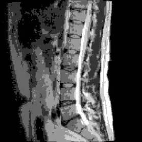
We start with a greyscale (150x150) image:

Let's see how many grey levels are there when representing the image in 8 bits:

ac = ImageData[ImageTake[i, All, All], "Byte"];
First@Dimensions@Tally@Flatten@ac
-> 234

Ok. Let's reduce those 234 levels. Our first try will be to let the algorithm alone to determine how many clusters are there with the default configuration:

ic = ClusteringComponents[Image@ac];
First@Dimensions@Tally@Flatten@ic 
-> 3

It selects 3 clusters, and the corresponding image is:

Now, if that is ok, or you need more clusters, is up to you.

Let's suppose you decide that a more fine-grained color separation is needed. Let's ask for 6 clusters instead of 3:

ic2 = ClusteringComponents[Image@ac, 6];
Image@ic2 // ImageAdjust  

Result:

and here are the pixel ranges used in each bin:

Table[{Min@#, Max@#} &@(Take[orig, {#[[1]]}, {#[[2]]}] & /@ 
    Position[clus, n]), {n, 1, 6}]
-> {{0, 11}, {12, 30}, {31, 52}, {53, 85}, {86, 134}, {135, 241}}

and the number of pixels in each bin:

Table[Count[Flatten@clus, i], {i, 6}]
-> {8906, 4400, 4261, 2850, 1363, 720}

So, the answer is YES, and it is straightforward.

Edit

Perhaps this will help you understand what you are doing wrong in your new example.

If I clusterize your color image, and use the cluster number to represent brightness, I get:

That's because the clusters are not being numbered in an ascending brightness order.

But if I calculate the mean brightness value for each cluster, and use it to represent the cluster value, I get:

In my previous example, that was not needed, but that was just luck :D (i.e. clusters were found in ascending brightness order)

Answer 2

k-means could be applied to your problem. If it were me, I would first try a basic approach borrowed from decision trees (although "simpler" is dependent upon your precise clustering algorithm!)

Assume one bin exists, begin stuffing the pixel intensities into the bin. When the bin is "full enough", compute the mean and standard deviation of the bin (or node). If the standard deviation is greater than some threshold, split the node in half. Continue this process until all intensities are done, and you will have a more efficient histogram.

This method can be improved with additional details of course:

1. You might consider using kurtosis as a splitting criteria.
2. Skewness might be used to determine where the split occurs
3. You might cross all the way into decision tree land and borrow the Jini index to guide splitting (some split techniques rely on more "exotic" statistics, like the t-test).
4. Lastly, you might perform a final consolidation pass to collapse any sparsely populated nodes.

Of course, if you've applied all of the above "improvements", then you've basically implemented one variation of a k-means clustering algorithm ;-)

Note: I disagree with the comment above - the problem you describe does not appear closely related histogram equalization.