Combine Line and Headmap plots in R

Question

on my research on how to plot multiple line charts I came across the following paper:

https://arxiv.org/pdf/1808.06019.pdf

It is showing a way on how huge amount of time series data is displayed by combining every line chart with a common headmap, the result looks like kind of equal to this representation:

DenseLines

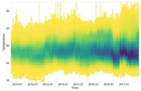
I was looking for an R package (but could not find anything) or a nice implementation for ggplot to achieve the same result. So I am able to plot a lot of geom_lines and color them differently but I do not know how to actually apply the headmap to it.

Does anyone has a hint/idea for me?

Thanks! Stephan

[See here](https://stackoverflow.com/questions/5963269/how-to-make-a-great-r-reproducible-example) on making an R question that folks can help with. That includes a sample of data, all necessary code, and a clear explanation of what you're trying to do and what hasn't worked. Right now this is a very broad question without a *specific* task. — camille, May 09 '19 at 21:20

Jon Spring · Accepted Answer · 2019-05-09T21:52:32.223

library(tidyverse)
datasets::ChickWeight # from Base R
ggplot(ChickWeight, aes(Time, weight, group = Chick)) + geom_line()

The wrangling here counts how many readings in each time / weight bucket, and normalizes to "share of most common reading" for each Time.

ChickWeight %>%
  count(Time, weight = 10*floor(weight/10)) %>%
  complete(Time, weight = 10*0:30, fill = list(n = 0)) %>%
  group_by(Time) %>%
  mutate(share = n / max(n)) %>%  # weighted for num as % of max for that Time
  ungroup() %>%

  ggplot(aes(Time, weight, fill = share)) +
  geom_tile(width = 2) +
  scale_fill_viridis_c(direction = -1)

If your data has sparse time readings, it might be useful to interpolate your lines to get more resolution for binning:

ChickWeight %>%
  group_by(Chick) %>%
  arrange(Time) %>%
  padr::pad_int("Time", step = 0.5) %>%
  mutate(weight_approx = approx(Time, weight, Time)$y) %>%
  ungroup() %>%

  count(Time, weight_approx = 10*floor(weight_approx/10)) %>%
  complete(Time, weight_approx = 10*0:60, fill = list(n = 0)) %>%
  group_by(Time) %>%
  mutate(share = n / sum(n)) %>%   # Different weighting option
  ungroup() %>%

  ggplot(aes(Time, weight_approx, fill = share)) +
  geom_tile() +
  scale_fill_viridis_c(direction = -1)

Hi Jon, thanks for the great (and super fast) answer! – Stephan Claus May 09 '19 at 21:51 — Stephan Claus, May 09 '19 at 21:51

Combine Line and Headmap plots in R

1 Answers1