How to overlay several plots

Question

I would like to plot in one graph 3 different occupancy patterns: a.) when both male and female are working; b.) only male working; c.) only female working.

I created 3 different data.frames using facet

The structure of the first data.frame (both male and female is working) is:

   structure(list(time = c("04:00", "04:15", "04:30", "04:45", "05:00", 
"05:15", "05:30", "05:45", "06:00", "06:15", "06:30", "06:45", 
"07:00", "07:15", "07:30", "07:45", "08:00", "08:15", "08:30", 
"08:45", "09:00", "09:15", "09:30", "09:45", "10:00", "10:15", 
"10:30", "10:45", "11:00", "11:15"), day = c("Monday", "Monday", 
"Monday", "Monday", "Monday", "Monday", "Monday", "Monday", "Monday", 
"Monday", "Monday", "Monday", "Monday", "Monday", "Monday", "Monday", 
"Monday", "Monday", "Monday", "Monday", "Monday", "Monday", "Monday", 
"Monday", "Monday", "Monday", "Monday", "Monday", "Monday", "Monday"
), variable = structure(c(1L, 1L, 1L, 1L, 1L, 1L, 1L, 1L, 1L, 
1L, 1L, 1L, 1L, 1L, 1L, 1L, 1L, 1L, 1L, 1L, 1L, 1L, 1L, 1L, 1L, 
1L, 1L, 1L, 1L, 1L), .Label = c("Shifts on Monday", "Shifts on Tuesday", 
"Shifts on Wednesday", "Shifts on Thursday", "Shifts on Friday", 
"Shifts on Saturday", "Shifts on Sunday"), class = "factor"), 
    value = c(102, 110, 116, 120, 148, 152, 188, 204, 318, 348, 
    418, 442, 752, 816, 1064, 1144, 1836, 1942, 2402, 2524, 3240, 
    3324, 3486, 3520, 3594, 3592, 3596, 3568, 3594, 3626), size_f = structure(c(1L, 
    1L, 1L, 1L, 1L, 1L, 1L, 1L, 1L, 1L, 1L, 1L, 1L, 1L, 1L, 1L, 
    1L, 1L, 1L, 1L, 1L, 1L, 1L, 1L, 1L, 1L, 1L, 1L, 1L, 1L), .Label = c("Monday", 
    "Tuesday", "Wednesday", "Thursday", "Friday", "Saturday", 
    "Sunday"), class = "factor")), row.names = c(NA, 30L), class = "data.frame")

The structure of the second data.frame (male is working) is:

dput(head(melted_WkSTiWeekM , 30))
structure(list(time = c("04:00", "04:15", "04:30", "04:45", "05:00", 
"05:15", "05:30", "05:45", "06:00", "06:15", "06:30", "06:45", 
"07:00", "07:15", "07:30", "07:45", "08:00", "08:15", "08:30", 
"08:45", "09:00", "09:15", "09:30", "09:45", "10:00", "10:15", 
"10:30", "10:45", "11:00", "11:15"), day = c("Monday", "Monday", 
"Monday", "Monday", "Monday", "Monday", "Monday", "Monday", "Monday", 
"Monday", "Monday", "Monday", "Monday", "Monday", "Monday", "Monday", 
"Monday", "Monday", "Monday", "Monday", "Monday", "Monday", "Monday", 
"Monday", "Monday", "Monday", "Monday", "Monday", "Monday", "Monday"
), variable = structure(c(1L, 1L, 1L, 1L, 1L, 1L, 1L, 1L, 1L, 
1L, 1L, 1L, 1L, 1L, 1L, 1L, 1L, 1L, 1L, 1L, 1L, 1L, 1L, 1L, 1L, 
1L, 1L, 1L, 1L, 1L), .Label = c("Shifts on Monday", "Shifts on Tuesday", 
"Shifts on Wednesday", "Shifts on Thursday", "Shifts on Friday", 
"Shifts on Saturday", "Shifts on Sunday"), class = "factor"), 
    value = c(56, 58, 64, 68, 84, 84, 104, 114, 172, 196, 224, 
    238, 410, 442, 560, 604, 930, 968, 1188, 1230, 1576, 1620, 
    1692, 1706, 1740, 1746, 1752, 1740, 1736, 1756), size_f = structure(c(1L, 
    1L, 1L, 1L, 1L, 1L, 1L, 1L, 1L, 1L, 1L, 1L, 1L, 1L, 1L, 1L, 
    1L, 1L, 1L, 1L, 1L, 1L, 1L, 1L, 1L, 1L, 1L, 1L, 1L, 1L), .Label = c("Monday", 
    "Tuesday", "Wednesday", "Thursday", "Friday", "Saturday", 
    "Sunday"), class = "factor")), row.names = c(NA, 30L), class = "data.frame")

The structure of the second data.frame (female is working) is:

structure(list(time = c("04:00", "04:15", "04:30", "04:45", "05:00", 
"05:15", "05:30", "05:45", "06:00", "06:15", "06:30", "06:45", 
"07:00", "07:15", "07:30", "07:45", "08:00", "08:15", "08:30", 
"08:45", "09:00", "09:15", "09:30", "09:45", "10:00", "10:15", 
"10:30", "10:45", "11:00", "11:15"), day = c("Monday", "Monday", 
"Monday", "Monday", "Monday", "Monday", "Monday", "Monday", "Monday", 
"Monday", "Monday", "Monday", "Monday", "Monday", "Monday", "Monday", 
"Monday", "Monday", "Monday", "Monday", "Monday", "Monday", "Monday", 
"Monday", "Monday", "Monday", "Monday", "Monday", "Monday", "Monday"
), variable = structure(c(1L, 1L, 1L, 1L, 1L, 1L, 1L, 1L, 1L, 
1L, 1L, 1L, 1L, 1L, 1L, 1L, 1L, 1L, 1L, 1L, 1L, 1L, 1L, 1L, 1L, 
1L, 1L, 1L, 1L, 1L), .Label = c("Shifts on Monday", "Shifts on Tuesday", 
"Shifts on Wednesday", "Shifts on Thursday", "Shifts on Friday", 
"Shifts on Saturday", "Shifts on Sunday"), class = "factor"), 
    value = c(46, 52, 52, 52, 64, 68, 84, 90, 146, 152, 194, 
    204, 342, 374, 504, 540, 906, 974, 1214, 1294, 1664, 1704, 
    1794, 1814, 1854, 1846, 1844, 1828, 1858, 1870), size_f = structure(c(1L, 
    1L, 1L, 1L, 1L, 1L, 1L, 1L, 1L, 1L, 1L, 1L, 1L, 1L, 1L, 1L, 
    1L, 1L, 1L, 1L, 1L, 1L, 1L, 1L, 1L, 1L, 1L, 1L, 1L, 1L), .Label = c("Monday", 
    "Tuesday", "Wednesday", "Thursday", "Friday", "Saturday", 
    "Sunday"), class = "factor")), row.names = c(NA, 30L), class = "data.frame")

After this I created a

melted_WkSTiWeekAll=cbind(melted_WkSTiWeek,melted_WkSTiWeekM,melted_WkSTiWeekF)



structure(list(time = c("04:00", "04:15", "04:30", "04:45", "05:00"
), day = c("Monday", "Monday", "Monday", "Monday", "Monday"), 
    variable = structure(c(1L, 1L, 1L, 1L, 1L), .Label = c("Shifts on Monday", 
    "Shifts on Tuesday", "Shifts on Wednesday", "Shifts on Thursday", 
    "Shifts on Friday", "Shifts on Saturday", "Shifts on Sunday"
    ), class = "factor"), value = c(102, 110, 116, 120, 148), 
    size_f = structure(c(1L, 1L, 1L, 1L, 1L), .Label = c("Monday", 
    "Tuesday", "Wednesday", "Thursday", "Friday", "Saturday", 
    "Sunday"), class = "factor"), time = c("04:00", "04:15", 
    "04:30", "04:45", "05:00"), day = c("Monday", "Monday", "Monday", 
    "Monday", "Monday"), variable = structure(c(1L, 1L, 1L, 1L, 
    1L), .Label = c("Shifts on Monday", "Shifts on Tuesday", 
    "Shifts on Wednesday", "Shifts on Thursday", "Shifts on Friday", 
    "Shifts on Saturday", "Shifts on Sunday"), class = "factor"), 
    value = c(56, 58, 64, 68, 84), size_f = structure(c(1L, 1L, 
    1L, 1L, 1L), .Label = c("Monday", "Tuesday", "Wednesday", 
    "Thursday", "Friday", "Saturday", "Sunday"), class = "factor"), 
    time = c("04:00", "04:15", "04:30", "04:45", "05:00"), day = c("Monday", 
    "Monday", "Monday", "Monday", "Monday"), variable = structure(c(1L, 
    1L, 1L, 1L, 1L), .Label = c("Shifts on Monday", "Shifts on Tuesday", 
    "Shifts on Wednesday", "Shifts on Thursday", "Shifts on Friday", 
    "Shifts on Saturday", "Shifts on Sunday"), class = "factor"), 
    value = c(46, 52, 52, 52, 64), size_f = structure(c(1L, 1L, 
    1L, 1L, 1L), .Label = c("Monday", "Tuesday", "Wednesday", 
    "Thursday", "Friday", "Saturday", "Sunday"), class = "factor")), row.names = c(NA, 
5L), class = "data.frame")

The variable time, day, variable and size_f are similar.

I would like to plot 3 graph together in the same plot. But I have no clue how to this

Using the suggested facet the following plot

Plot1

Plot2

Plot3

How to move forward

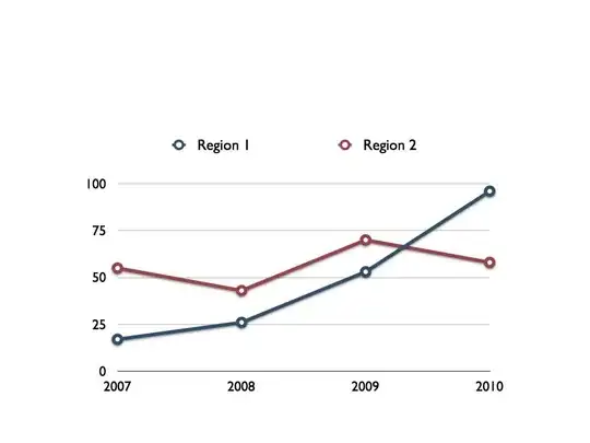
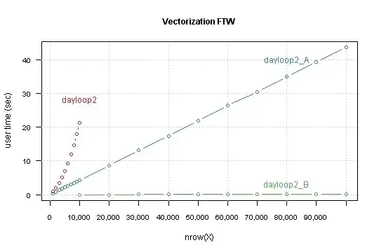
I would like to create a pot like this

@qwr I managed to create individual graphs how to overlay the plot? — user11418708, May 30 '19 at 22:36
@M-M thanks , any suggestion how to continue, I am working on this idea https://stackoverflow.com/questions/44066444/how-to-plot-the-difference-between-two-density-distributions?rq=1 — user11418708, May 30 '19 at 22:45
@user11418708 do you want to combine all the facets (all days of weeks) into one plot overlaying each other or have different plot for each day but combine your 3 different plots and have 3 densities on each facet? — M--, May 30 '19 at 22:49
@ M-M thanks for your reply; i don't want densities - but I want the plot to be similar to the densities -> basically I just want to overlay all 3 plots to show their intersection -> to show the daily working aptterns of males and females — user11418708, May 30 '19 at 22:51
```library(tidyverse); melted_WkSTiWeekAll <- bind_rows(list(All=melted_WkSTiWeek,Male=melted_WkSTiWeekM,Female=melted_WkSTiWeekF), .id = 'source'); ggplot(melted_WkSTiWeekAll ,aes(x=time,y=value,fill=source)) + geom_bar(stat="identity",position = "identity", alpha=.3, width=1) + facet_wrap(~day)``` — M--, May 31 '19 at 00:00

M-- · Accepted Answer · 2022-02-07T17:13:10.563

You can do it by merging your dataframes together and tag them as All, Male, and Female accordingly. Then you can use that tag for grouping(coloring) within your ggplot function.

Using geom_bar and position = "identity" you will get bars on top of each other and to remove the space between the bars (to mimic density plots look) width is set to 1. alpha can be used to alter the transparency of fill colors.

And to get a separate plot for each day of the week we can use facet_wrap(~day).

library(tidyverse)

melted_WkSTiWeekAll <- bind_rows(list(All=melted_WkSTiWeek,
                                      Male=melted_WkSTiWeekM,
                                      Female=melted_WkSTiWeekF), 
                                                                .id = 'source')

ggplot(melted_WkSTiWeekAll, aes(x=time, y=value, fill=source)) + 
  geom_bar(stat="identity", position = "identity", alpha=.3, width=1) + 
  facet_wrap(~day)

^{Note that here we only get one facet as the data provided only has entries for Monday.} ^{Created on 2019-05-31 by the reprex package (v0.3.0)}

How to overlay several plots

1 Answers1