barchart - axis ticks are not adjusted according to the bars

Question

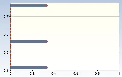
I have to draw a bar chart in R ggplot2 with multiple variables (i.e each bar for BMI, weight, cholesterol, Blood pressure etc) in each group ( i.e. different populations ex: Indian, Korean, Philipinos etc.) But the bars are overflowing to the next group in the axis. for example: the bars of the Indian group is overflowing to Korean group. The axis marks are not adjusted accordingly. I have attached the figure .. can someone please help. Following is my code. dput(data) is also given.

p = ggplot(data = t, 
           aes(x = factor(Population, levels = names(sort(table(Population), increasing = TRUE))),
               y = Snp_Count, 
               group = factor(Trait, levels = c("BMI", "DBP", "HDL", "Height", "LDL", "TC", "TG", "WC", "Weight"), 
                              ordered = TRUE)))

p = p + geom_bar(aes(fill = Trait), 
                 position = position_dodge(preserve = "single"), 
                 stat = "identity") + 
  scale_fill_manual(values = c("#28559A", "#3EB650", "#E56B1F", "#A51890", "#FCC133", "#663300", "#6666ff", "#ff3300", "#ff66ff")) + 
  coord_flip()

structure(list(Trait = structure(c(1L, 1L, 1L, 1L, 1L, 1L, 1L, 
1L, 1L, 1L, 1L, 1L, 2L, 2L, 2L, 2L, 3L, 3L, 3L, 3L, 3L, 3L, 3L, 
3L, 3L, 3L, 3L, 3L, 3L, 3L, 3L, 3L, 4L, 4L, 4L, 4L, 5L, 5L, 5L, 
5L, 5L, 5L, 5L, 5L, 5L, 5L, 5L, 6L, 6L, 6L, 6L, 6L, 6L, 6L, 7L, 
7L, 7L, 7L, 7L, 7L, 7L, 7L, 7L, 7L, 7L, 7L, 7L, 7L, 7L, 7L, 7L, 
7L, 8L, 8L, 8L, 8L, 8L, 8L, 8L, 9L, 9L, 9L, 9L, 9L, 9L, 9L), .Label = c("BMI", 
"DBP", "HDL", "HT", "LDL", "TC", "TG", "WC", "Weight"), class = "factor"), 
    Association = structure(c(1L, 1L, 1L, 1L, 1L, 1L, 1L, 1L, 
    1L, 1L, 1L, 1L, 1L, 1L, 1L, 1L, 1L, 1L, 1L, 1L, 1L, 1L, 1L, 
    1L, 1L, 1L, 1L, 1L, 1L, 1L, 1L, 1L, 1L, 1L, 1L, 1L, 1L, 1L, 
    1L, 1L, 1L, 1L, 1L, 1L, 1L, 1L, 1L, 1L, 1L, 1L, 1L, 1L, 1L, 
    1L, 1L, 1L, 1L, 1L, 1L, 1L, 1L, 1L, 1L, 1L, 1L, 1L, 1L, 1L, 
    1L, 1L, 1L, 1L, 1L, 1L, 1L, 1L, 1L, 1L, 1L, 1L, 1L, 1L, 1L, 
    1L, 1L, 1L), .Label = "Direct", class = "factor"), TraitClass = structure(c(1L, 
    1L, 1L, 1L, 1L, 1L, 1L, 1L, 1L, 1L, 1L, 1L, 2L, 2L, 2L, 2L, 
    3L, 3L, 3L, 3L, 3L, 3L, 3L, 3L, 3L, 3L, 3L, 3L, 3L, 3L, 3L, 
    3L, 1L, 1L, 1L, 1L, 3L, 3L, 3L, 3L, 3L, 3L, 3L, 3L, 3L, 3L, 
    3L, 3L, 3L, 3L, 3L, 3L, 3L, 3L, 3L, 3L, 3L, 3L, 3L, 3L, 3L, 
    3L, 3L, 3L, 3L, 3L, 3L, 3L, 3L, 3L, 3L, 3L, 1L, 1L, 1L, 1L, 
    1L, 1L, 1L, 1L, 1L, 1L, 1L, 1L, 1L, 1L), .Label = c("Anthropometric", 
    "BP", "Lipid"), class = "factor"), Population = structure(c(2L, 
    3L, 4L, 5L, 7L, 8L, 10L, 11L, 12L, 13L, 22L, 24L, 3L, 5L, 
    11L, 22L, 3L, 4L, 5L, 6L, 7L, 8L, 9L, 10L, 11L, 12L, 13L, 
    14L, 15L, 18L, 20L, 28L, 5L, 7L, 13L, 14L, 1L, 3L, 5L, 7L, 
    9L, 11L, 12L, 16L, 18L, 20L, 22L, 5L, 6L, 7L, 10L, 12L, 18L, 
    20L, 3L, 5L, 6L, 7L, 8L, 11L, 12L, 13L, 14L, 15L, 18L, 19L, 
    20L, 21L, 22L, 23L, 26L, 28L, 3L, 4L, 5L, 8L, 12L, 22L, 24L, 
    3L, 5L, 7L, 8L, 17L, 25L, 27L), .Label = c("ACB", "AFR", 
    "ASW", "ASW/ACB", "CEU", "CHB", "EAS", "Filipino", "FIN", 
    "GBR", "Hispanic", "Hispanic/Latinos", "JPT", "Korean", "Kuwaiti", 
    "Micronesian", "Moroccan", "MXL", "Mylopotamos", "Orcadian", 
    "Pomak", "SAS", "Saudi_Arabian", "Seychellois", "Surinamese", 
    "Taiwanese", "Turkish", "YRI"), class = "factor"), Snp_Count = c(3L, 
    12L, 6L, 17L, 2L, 10L, 1L, 6L, 3L, 3L, 10L, 6L, 1L, 1L, 1L, 
    1L, 2L, 1L, 10L, 1L, 1L, 2L, 1L, 2L, 1L, 1L, 3L, 1L, 1L, 
    2L, 1L, 2L, 20L, 5L, 4L, 1L, 1L, 2L, 7L, 2L, 1L, 1L, 1L, 
    1L, 1L, 1L, 2L, 8L, 2L, 4L, 3L, 1L, 2L, 1L, 4L, 20L, 5L, 
    11L, 2L, 4L, 3L, 4L, 2L, 3L, 4L, 1L, 1L, 1L, 2L, 2L, 1L, 
    2L, 3L, 2L, 4L, 4L, 1L, 4L, 2L, 2L, 2L, 1L, 1L, 1L, 1L, 1L
    ), Gene_Count = c(3L, 9L, 7L, 9L, 2L, 8L, 1L, 7L, 3L, 2L, 
    8L, 7L, 1L, 1L, 1L, 1L, 2L, 1L, 4L, 1L, 1L, 1L, 1L, 2L, 2L, 
    1L, 2L, 1L, 1L, 1L, 1L, 1L, 9L, 6L, 5L, 1L, 1L, 2L, 5L, 2L, 
    1L, 1L, 1L, 1L, 1L, 1L, 2L, 6L, 2L, 3L, 3L, 1L, 2L, 1L, 3L, 
    10L, 4L, 7L, 1L, 3L, 3L, 4L, 1L, 3L, 5L, 1L, 1L, 1L, 3L, 
    3L, 1L, 1L, 2L, 2L, 3L, 3L, 1L, 3L, 2L, 3L, 3L, 2L, 3L, 2L, 
    2L, 2L)), class = "data.frame", row.names = c(NA, -86L))

I guess the problem lies in the `preserve = "single`, but without a reproducible example it is hard to tell. Please share your data with `dput` or something similar. — kath, Jul 11 '19 at 08:24
I ran the code with your data and I can't reproduce the issue, the groups are nicely separated in my plot — kath, Jul 11 '19 at 08:37
Sorry kath it happend when i tried to increase the width of the bars... `p=ggplot(data=t,aes(x=factor(Population,levels=names(sort(table(Population),increasing=TRUE))), y=Snp_Count, group=factor(Trait,levels=c("BMI","DBP","HDL","Height","LDL","TC","TG","WC","Weight"), ordered=TRUE)))` `p <- p+geom_bar(aes(fill=Trait), ***width=3***, position=position_dodge2(preserve= c("single")), stat="identity") + scale_fill_manual(values=c("#28559A","#3EB650","#E56B1F","#A51890","#FCC133","#663300","#6666ff","#ff3300","#ff66ff")) + coord_flip()` — arshad, Jul 11 '19 at 08:44
I see... that won't work. I'll write up an answer with some suggestions. — kath, Jul 11 '19 at 08:50
Related question: https://stackoverflow.com/questions/33877720/what-units-are-the-width-in-geom-baraes-and-position-dodgewidth-r — kath, Jul 11 '19 at 09:30

kath · Accepted Answer · 2019-07-11T09:35:51.430

The total width of each group in your barchart is 0.9 by default, which means that 90% of the area is covered. When you increase the width of the individual bars to 3 they will overlap with other groups, the maximum value for with should thus be 1 and then it will touch the other groups.

I'd suggest in your situation to use facet_wrap instead of a dodged barchart.

Note: geom_col is the same as geom_bar(stat = "identity).

my.df$Trait <- factor(my.df$Trait, levels = c("BMI", "DBP", "HDL", "HT", "LDL", "TC", "TG", "WC", "Weight"))
my.df$Population <- factor(my.df$Population, levels = names(sort(table(my.df$Population), increasing = TRUE)))

ggplot(my.df, aes(x = Trait, y = Snp_Count, fill = Trait)) + 
  geom_col(width = 1) +
  scale_fill_manual(values = c("#28559A", "#3EB650", "#E56B1F", "#A51890", "#FCC133", "#663300", "#6666ff", "#ff3300", "#ff66ff")) + 
  # Split the data by Population, allow flexible scales and spacing for y axis (Trait)
  facet_grid(Population ~ ., scales = "free_y", space = "free_y", switch = "y") +
  coord_flip() +
  theme(axis.text.y = element_blank(), # Remove Trait labels (indicated by color)
        axis.ticks.y = element_blank(), # Remove tick marks
        strip.background = element_blank(), 
        strip.text.y = element_text(angle = 180, hjust = 1), # Rotate Population labels
        panel.spacing.y = unit(3, "pt")) # Spacing between groups

Data

my.df <- 
  structure(list(Trait = structure(c(1L, 1L, 1L, 1L, 1L, 1L, 1L, 
                                     1L, 1L, 1L, 1L, 1L, 2L, 2L, 2L, 2L, 3L, 3L, 3L, 3L, 3L, 3L, 3L, 
                                     3L, 3L, 3L, 3L, 3L, 3L, 3L, 3L, 3L, 4L, 4L, 4L, 4L, 5L, 5L, 5L, 
                                     5L, 5L, 5L, 5L, 5L, 5L, 5L, 5L, 6L, 6L, 6L, 6L, 6L, 6L, 6L, 7L, 
                                     7L, 7L, 7L, 7L, 7L, 7L, 7L, 7L, 7L, 7L, 7L, 7L, 7L, 7L, 7L, 7L, 
                                     7L, 8L, 8L, 8L, 8L, 8L, 8L, 8L, 9L, 9L, 9L, 9L, 9L, 9L, 9L), 
                                   .Label = c("BMI", "DBP", "HDL", "HT", "LDL", "TC", "TG", "WC", "Weight"), class = "factor"), 
                 Population = structure(c(2L, 3L, 4L, 5L, 7L, 8L, 10L, 11L, 
                                          12L, 13L, 22L, 24L, 3L, 5L, 11L, 22L, 3L, 4L, 5L, 6L, 7L, 
                                          8L, 9L, 10L, 11L, 12L, 13L, 14L, 15L, 18L, 20L, 28L, 5L, 
                                          7L, 13L, 14L, 1L, 3L, 5L, 7L, 9L, 11L, 12L, 16L, 18L, 20L, 
                                          22L, 5L, 6L, 7L, 10L, 12L, 18L, 20L, 3L, 5L, 6L, 7L, 8L, 
                                          11L, 12L, 13L, 14L, 15L, 18L, 19L, 20L, 21L, 22L, 23L, 26L, 
                                          28L, 3L, 4L, 5L, 8L, 12L, 22L, 24L, 3L, 5L, 7L, 8L, 17L, 
                                          25L, 27L), 
                                        .Label = c("ACB", "AFR", "ASW", "ASW/ACB", "CEU", 
                                                   "CHB", "EAS", "Filipino", "FIN", "GBR", "Hispanic", "Hispanic/Latinos", 
                                                   "JPT", "Korean", "Kuwaiti", "Micronesian", "Moroccan", "MXL", 
                                                   "Mylopotamos", "Orcadian", "Pomak", "SAS", "Saudi_Arabian", 
                                                   "Seychellois", "Surinamese", "Taiwanese", "Turkish", "YRI"), class = "factor"), 
                 Snp_Count = c(3L, 12L, 6L, 17L, 2L, 
                               10L, 1L, 6L, 3L, 3L, 10L, 6L, 1L, 1L, 1L, 1L, 2L, 1L, 10L, 
                               1L, 1L, 2L, 1L, 2L, 1L, 1L, 3L, 1L, 1L, 2L, 1L, 2L, 20L, 
                               5L, 4L, 1L, 1L, 2L, 7L, 2L, 1L, 1L, 1L, 1L, 1L, 1L, 2L, 8L, 
                               2L, 4L, 3L, 1L, 2L, 1L, 4L, 20L, 5L, 11L, 2L, 4L, 3L, 4L, 
                               2L, 3L, 4L, 1L, 1L, 1L, 2L, 2L, 1L, 2L, 3L, 2L, 4L, 4L, 1L, 
                               4L, 2L, 2L, 2L, 1L, 1L, 1L, 1L, 1L)), 
            class = "data.frame", row.names = c(NA, -86L))

barchart - axis ticks are not adjusted according to the bars

1 Answers1