Multivariate curve-fitting in python for estimating the parameter and order of ellipse-like shapes

Question

I'm trying to find the best parameters (a, b, and c) of the following function (general formula of circle, ellipse, or rhombus):

                       (|x|/a)^c + (|y|/b)^c = 1

of two arrays of independent data (x and y) in python. My main objective is to estimate the best value of (a, b, and c) based on my x and y variable. I am using curve_fit function from scipy, so here is my code with a demo x, and y.

import numpy as np
import matplotlib.pyplot as plt
from scipy.optimize import curve_fit

alpha = 5
beta = 3
N = 500
DIM = 2

np.random.seed(2)

theta = np.random.uniform(0, 2*np.pi, (N,1))
eps_noise = 0.2 * np.random.normal(size=[N,1])
circle = np.hstack([np.cos(theta), np.sin(theta)])

B = np.random.randint(-3, 3, (DIM, DIM))
noisy_ellipse = circle.dot(B) + eps_noise

X = noisy_ellipse[:,0:1]
Y = noisy_ellipse[:,1:]

def func(xdata, a, b,c):
    x, y = xdata
    return (np.abs(x)/a)**c + (np.abs(y)/b)**c

xdata = np.transpose(np.hstack((X, Y)))
ydata = np.ones((xdata.shape[1],))

pp, pcov = curve_fit(func, xdata, ydata, maxfev = 1000000, bounds=((0, 0, 1), (50, 50, 2)))

plt.scatter(X, Y, label='Data Points')
x_coord = np.linspace(-5,5,300)
y_coord = np.linspace(-5,5,300)
X_coord, Y_coord = np.meshgrid(x_coord, y_coord)
Z_coord = func((X_coord,Y_coord),pp[0],pp[1],pp[2])
plt.contour(X_coord, Y_coord, Z_coord, levels=[1], colors=('g'), linewidths=2)
plt.legend()
plt.xlabel('X')
plt.ylabel('Y')
plt.show()

By using this code, the parameters are [4.69949891, 3.65493859, 1.0] for a, b, and c.

The problem is that I usually get the value of c the smallest in its bound, while in this demo data it (i.e., c parameter) supposes to be very close to 2 as the data represent an ellipse.

Any help and suggestions for solving this issue are appreciated.

Answer 1

A curve which equation is (|x/a|)^c + (|y/b|)^c = 1 is called "Superellipse" : http://mathworld.wolfram.com/Superellipse.html

For large c the superellipse tends to a rectangular shape.

For c=2 the curve is an ellipse, or a circle in the particular case a=b.

For c close to 1 the superellipse tends to a rhombus shape.

For c larger than 0 and lower than 1 the superellipse looks like a (squashed) astroid with sharp vertices. This kind of shape will not be considered below.

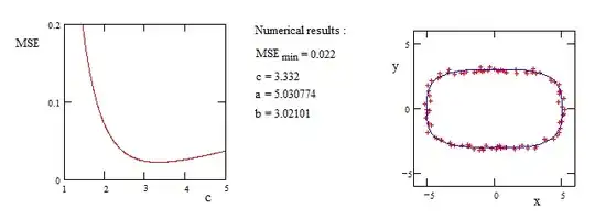
Before looking to the right question of the OP, it is of interest to study the regression behaviour for fitting a superellipse to scattered data. A short experimental and simplified approach tends to make understand the mathematical difficulty, prior the programming difficulties.

When the scatter increases the computed value of c (corresponding to the minimum of MSE ) decreases. Also the minimum becomes more and more difficult to localize. This is certainly a difficulty for the softwares.

For even larger scatter the value of c=1 leads to a rhombus shape.

So, it is not surprizing that in the example highly scattered published by the OP the software gave a rhombus as fitted curve.

If this was not the expected result, one have to chose another goal than the minimum MSE. For example if the goal is to obtain an elliptic shape, one have to set c=2. The result on the next figure shows that the MSE is worse than with the preceeding rhombus shape. But the elliptic fitting is well achieved.

NOTE : In case of large scatter the result depends a lot from the choice of criteria of fitting (MSE, MAE, ..., and with respect to what variable). This can be the cause of very different results from a software to another if the criterias of fitting (sometime not explicit) are different.

Among the criterias of fitting, if it is specified that the rhombus shape is excluded, one have to define more representative criteria and/or model and implement them in the software.

IMPORTANCE OF CRITERIA OF FITTING :

In order to show how the choice of criteria of fitting is important especially in case of data highly scattered, we will make the study again with a different criteria.

Instead of the preceeding criteria which was the MSE of the errors on the superellipse equation itself, that was :

we chose a different criteria, for example the MSE of the errors on the radial coordinate in polar system :

The notations are defined on the next picture :

Some results from the empirical study for increasing scatter :

We observe that the numerical calculus with the second criteria is more robust that with the first. Cases with higher scatter can be treated With the second criteria of fitting .

The drawback it that this second criteria is probably not considered in the available softwares. So one have to implement the above formulas in the existing software if possible. Or to write a software especially adapted.

Nevertheless this discussion about criteria of fitting is somehow out of subject because the criteria of fitting should not result from mathematical considerations only. If the problem comes from a practical need in physic or technology the criteria of fitting might be derived from the reality without choice.

Answer 2

I have modified your code (though you took it from https://stackoverflow.com/a/47881806/10640534) quite a lot, but I think I have what you expect. I am using a different equation, which I found here. I have also used the new Numpy random generators, but I believe that is only aesthetic for this problem. I am drawing the ellipse using patches from matplotlib, which indeed is aesthetic, but definitely a way better solution to represent your conic. Importantly, I am using the dogbox method for curve_fit because other methods do not converge; occasionally the ellipse is not matched and decreasing the added noise (e.g., rng.normal(0, 1, (500, 2)) / 1e2 instead of rng.normal(0, 1, (500, 2)) / 1e1 helps). Anyway, snippet and figure below.

import numpy as np
from numpy.random import default_rng
from matplotlib.patches import Ellipse
import matplotlib.pyplot as plt
from scipy.optimize import curve_fit


def func(data, a, b, h, k, A):
    x, y = data
    return ((((x - h) * np.cos(A) + (y - k) * np.sin(A)) / a) ** 2
            + (((x - h) * np.sin(A) - (y - k) * np.cos(A)) / b) ** 2)


rng = default_rng(3)
numPoints = 500
center = rng.random(2) * 10 - 5
theta = rng.uniform(0, 2 * np.pi, (numPoints, 1))
circle = np.hstack([np.cos(theta), np.sin(theta)])
ellipse = (circle.dot(rng.random((2, 2)) * 2 * np.pi - np.pi)
           + (center[0], center[1]) + rng.normal(0, 1, (500, 2)) / 1e1)
pp, pcov = curve_fit(func, (ellipse[:, 0], ellipse[:, 1]), np.ones(numPoints),
                     p0=(1, 1, center[0], center[1], np.pi / 2),
                     method='dogbox')
plt.scatter(ellipse[:, 0], ellipse[:, 1], label='Data Points')
plt.gca().add_patch(Ellipse(xy=(pp[2], pp[3]), width=2 * pp[0],
                            height=2 * pp[1], angle=pp[4] * 180 / np.pi,
                            fill=False))
plt.gca().set_aspect('equal')
plt.tight_layout()
plt.show()

To incorporate the value of the exponent, I have used your equation and generated an ellipse according to this answer. This results in:

import numpy as np
from numpy.random import default_rng
from matplotlib.patches import Ellipse
import matplotlib.pyplot as plt
from scipy.optimize import curve_fit, root
from scipy.special import ellipeinc


def angles_in_ellipse(num, a, b):
    assert(num > 0)
    assert(a < b)
    angles = 2 * np.pi * np.arange(num) / num
    if a != b:
        e = (1.0 - a ** 2.0 / b ** 2.0) ** 0.5
        tot_size = ellipeinc(2.0 * np.pi, e)
        arc_size = tot_size / num
        arcs = np.arange(num) * arc_size
        res = root(lambda x: (ellipeinc(x, e) - arcs), angles)
        angles = res.x
    return angles


def func(data, a, b, c):
    x, y = data
    return (np.absolute(x) / a) ** c + (np.absolute(y) / b) ** c


a = 10
b = 20
n = 100
phi = angles_in_ellipse(n, a, b)
e = (1.0 - a ** 2.0 / b ** 2.0) ** 0.5
arcs = ellipeinc(phi, e)
noise = default_rng(0).normal(0, 1, n) / 2
pp, pcov = curve_fit(func, (b * np.sin(phi) + noise,
                            a * np.cos(phi) + noise),
                     np.ones(n), method='lm')
plt.scatter(b * np.sin(phi) + noise, a * np.cos(phi) + noise,
            label='Data Points')
plt.gca().add_patch(Ellipse(xy=(0, 0), width=2 * pp[0], height=2 * pp[1],
                            angle=0, fill=False))
plt.gca().set_aspect('equal')
plt.tight_layout()
plt.show()

As you decrease noise values, pp will tend to (b, a, 2).