How I can adjust the scale of axis X with breaks as.integer when I graph missing dates in R ggplot2

Question

How I can adjust the scales axis X in breaks as.integer when I have a lot of data graphing missing dates.

The code that I am using is the next (@Stefan Helped me):

#SET OF DATA
df <- read.table(text="
    Fecha - T - Tmin - Tmax
    2015-07-01 - 11,16 - 7,3 - 17
    2015-07-02 - 11,49 - 8 - 17,1
    2015-07-03 - 11,2 - 8,8 - 15,8
    2015-07-04 - 11,20 - 8,6 - 16
    2015-07-05 - 11,23 - 8,9 - 15,7
    2015-07-06 - 10,40 - 7,7 - 15,4
    2015-07-07 - 10,10 - 8,1 - 14,8
    2015-07-08 - 10,04 - 7,3 - 15,4
    2018-01-01 - 11,08 - 4,9 - 17,8
    2018-01-02 - 11,40 - 4,2 - 16,3
    2018-01-03 - 9,000 - 5,5 - 13,5
    2018-01-04 - 8,584 - 6 - 12,8
    2018-01-05 - 8,679 - 7,3 - 11,9
    2018-01-06 - 8,75 - 6,8 - 13
    2018-01-07 - 9,33 - 6,4 - 15,2
    2018-01-08 - 9,63 - 6,3 - 13,9
", header = TRUE, dec = ",")

INITIAL CODE

mmp1 <- df[,!grepl("^X", names(df))]
mmp1$Fecha <- as.Date(mmp1$Fecha)

library(ggplot2)
library(scales)
library(dplyr)
library(tibble)

mmp2 <- mmp1 %>% 
  mutate(
    year_fecha = as.character(lubridate::year(Fecha)),
    Fecha2 = format(Fecha, "%d-%m"),
    Fecha2 = forcats::fct_reorder(Fecha2, Fecha)) %>% 
  arrange(Fecha) %>% 
  rowid_to_column(var = "Fecha3")

# Put the theme code aside
polish <- theme(text = element_text(size=11)) +
  theme(axis.text.x=element_text(angle=45, hjust=1))+
  theme(plot.title = element_text(hjust = 0.5))+
  theme(panel.background = element_rect(fill = 'white', colour = 'white', size = 1.2, linetype = 7))+
  theme(text=element_text(family="arial", face="bold", size=12))+
  theme(axis.title.y = element_text(face="bold", family = "arial", vjust=1.5, colour="black", hjust = 0.5, size=rel(1.2)))+
  theme(axis.title.x = element_text(face="bold", family = "arial", vjust=0.5, colour="black", size=rel(1.2)))+
  theme(axis.text.x = element_text(family= "sans",face = "plain", colour="black", size=rel(1.1)))+
  theme(axis.text.y = element_text(family= "sans",face = "plain", colour="black", size=rel(1.1)))+
  theme(axis.line = element_line(size = 1, colour = "black"))+
  theme(legend.title = element_text(colour="black", size=12, face="bold", family = "arial"))+
  theme(legend.key = element_rect(fill = "white"))

# Simple and prefered solution: Facet by e.g. by year
w1 <- ggplot(data = mmp2) +
  geom_line(mapping = aes(x = Fecha, y = Tmin, colour="Min"), size=0.71) +
  geom_line(mapping = aes(x = Fecha, y = T, colour="P"), size=0.71) +
  geom_line(mapping = aes(x = Fecha, y = Tmax, colour="Max"), size=0.71) +
  scale_x_date(date_breaks = "1 day", date_labels = "%d-%m", expand = (c(0.001,0.008)))+
  scale_y_continuous(breaks=seq(-4, 28, 2), limits = c(1,18), expand=c(0,0)) +
  scale_colour_manual(name="Leyenda",
                      values=c(Min="green", P="#56B4E9", Max="Red")) +
  ylab("Temperatura (C)")+
  xlab("Tiempo") +
  guides(colour=guide_legend(order = 2),
         shape=guide_legend(order = 2)) +
  facet_wrap(~year_fecha, scales = "free_x") +
  polish

w1

The first result is:

First result is

# Hacky solutions with some manual labelling
labs <- select(mmp2, Fecha3, Fecha2) %>% 
  tibble::deframe()

date_lab <- function(x) {
  labs[as.character(x)]
}

# Draw the data as one continuous line
w2 <- ggplot(data = mmp2) +
  geom_line(mapping = aes(x = Fecha3, y = Tmin, colour="Min"), size=0.71) +
  geom_line(mapping = aes(x = Fecha3, y = T, colour="P"), size=0.71) +
  geom_line(mapping = aes(x = Fecha3, y = Tmax, colour="Max"), size=0.71) +
  scale_x_continuous(breaks = as.integer(names(labs)), labels = date_lab, expand = (c(0.001,0.008))) +
  scale_y_continuous(breaks=seq(-4, 28, 2), limits = c(1,18), expand=c(0,0)) +
  scale_colour_manual(name="Leyenda",
                      values=c(Min="green", P="#56B4E9", Max="Red")) +
  ylab("Temperatura (C)")+
  xlab("Tiempo") +
  guides(colour=guide_legend(order = 2),
         shape=guide_legend(order = 2)) +
  polish
w2

Second result is:

Second result

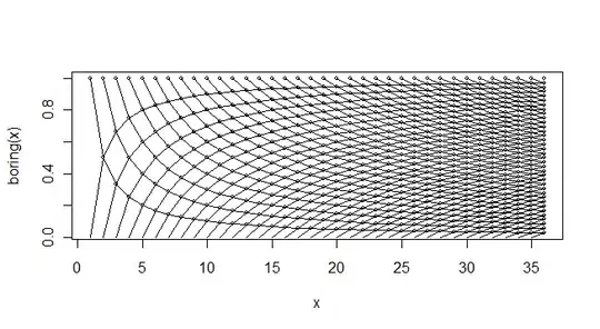
Using the same code but graphing a lot of data I have this problem:

Graph with many data

How I can adjust this axix X? Thank you.

Convert your x-axis to `Date` then use `scale_x_date` to control the breaks and labels. See these examples: https://stackoverflow.com/a/50710428/786542 & https://stackoverflow.com/q/56811184/786542 — Tung, Mar 28 '20 at 23:40
No, is not posible because in the last part of the code, is other format. — John_Erick, Mar 29 '20 at 00:51
Hi John_Erick. First. Please mark answers as accepted if they helped you to solve your problem. Second. When asking a second question: Instead of pasting the answer in your post simply put a link to the first question/answer in the post. Third. Instead of posting a second question you could have simply asked me to help you with the second problem. As I'm already familiar with the problem and the answer, it's probably much easier for me to adjust my answer. Fourth. See my answer to the second question. (: — stefan, Mar 29 '20 at 08:48
Thank you so much Stefan your help have been so big. I am new in this plataform and programing in R, and there are something that I don´t know. I did this question in the fisrt problem or question, but a moderator deleted twice my question, therefore I had to ask again. Thank you, I will put in practice your tips. — John_Erick, Mar 29 '20 at 13:02

score 0 · Accepted Answer · answered Mar 29 '20 at 09:06

First question was to remove the "gaps" in your data. As I said, the simplest solution would be facetting by e.g. year. This would allow you to work with a date scale.

Your second problem is related to the overplotting of labels. This kind of overplotting naturally arises with dates when trying to plot single days. With a lot of days, say one year or more it is simply not possible to label all days. The solution therefore is to restrict the days to plot. When working with a date scale this can be easily achieved via some helper function (e.g. breaks = breaks_width("1 week")).

To mimic this behaviour for the hacky solution I added this code:

breaks <- mmp2 %>% 
  # Plots first, 8th, 15th, ... of day of a month
  mutate(days_to_plot = lubridate::day(Fecha) %in% c(1, 8, 15, 22, 29)) %>% 
  filter(days_to_plot) %>% 
  pull(Fecha3)

This is not a perfect solution but it reduces the lables to plot considerably.

So try this with your large dataset:

library(ggplot2)
library(scales)
library(dplyr)
library(tibble)
library(lubridate)

mmp2 <- mmp1 %>% 
  mutate(
    year_fecha = as.character(lubridate::year(Fecha)),
    Fecha2 = format(Fecha, "%d-%m"),
    Fecha2 = forcats::fct_reorder(Fecha2, Fecha)) %>% 
  arrange(Fecha) %>% 
  rowid_to_column(var = "Fecha3")

# Put the seem code aside
polish <- theme(text = element_text(size=11)) +
  theme(axis.text.x=element_text(angle=45, hjust=1))+
  theme(plot.title = element_text(hjust = 0.5))+
  theme(panel.background = element_rect(fill = 'white', colour = 'white', size = 1.2, linetype = 7))+
  theme(text=element_text(family="sans", face="bold", size=12))+
  theme(axis.title.y = element_text(face="bold", family = "sans", vjust=1.5, colour="black", hjust = 0.5, size=rel(1.2)))+
  theme(axis.title.x = element_text(face="bold", family = "sans", vjust=0.5, colour="black", size=rel(1.2)))+
  theme(axis.text.x = element_text(family= "sans",face = "plain", colour="black", size=rel(1.1)))+
  theme(axis.text.y = element_text(family= "sans",face = "plain", colour="black", size=rel(1.1)))+
  theme(axis.line = element_line(size = 1, colour = "black"))+
  theme(legend.title = element_text(colour="black", size=12, face="bold", family = "arial"))+
  theme(legend.key = element_rect(fill = "white"))

# Draw the data as one continuous line
# Hacky solutions with some manual labelling
labs <- select(mmp2, Fecha3, Fecha2) %>% 
  tibble::deframe()

date_lab <- function(x) {
  labs[as.character(x)]
}

# Which detas/days should be shown on x-axis
breaks <- mmp2 %>% 
  # Plots first, 8th, 15th, ... of day of a month
  mutate(days_to_plot = day(Fecha) %in% c(1, 8, 15, 22, 29)) %>% 
  filter(days_to_plot) %>% 
  pull(Fecha3)

w4 <- ggplot(data = mmp2) +
  geom_line(mapping = aes(x = Fecha3, y = Tmin, colour="Min"), size=0.71) +
  geom_line(mapping = aes(x = Fecha3, y = T, colour="P"), size=0.71) +
  geom_line(mapping = aes(x = Fecha3, y = Tmax, colour="Max"), size=0.71) +
  scale_x_continuous(breaks = breaks, labels = date_lab, expand = (c(0.001,0.008))) +
  scale_y_continuous(breaks=seq(-4, 28, 2), limits = c(1,18), expand=c(0,0)) +
  scale_colour_manual(name="Leyenda",
                      values=c(Min="green", P="#56B4E9", Max="Red")) +
  ylab("Temperatura (C)")+
  xlab("Tiempo") +
  guides(colour=guide_legend(order = 2),
         shape=guide_legend(order = 2)) +
  polish
w4

^{Created on 2020-03-29 by the reprex package (v0.3.0)}

If you still have problems with overplotting, then increas the width between lables or try the new guide_axis function introduced in ggplot 3.3.0, e.g.

scale_x_continuous(breaks = breaks, labels = date_lab, expand = (c(0.001,0.008)), guide = guide_axis(n.dodge = 2))

will split the lables on two rows.

I have a question: If I have a format "%Y-%m-%d %H:%M", I will have a lot of dates on the axis x because for example anyday "2018-01-01 00:00, 2018-01-01 00:15, 2018-01-01 00:30.....2018-01-01 23:15". In this format, How can I get a appropriate breaks on the labels of X-axix? Thank you. — John_Erick, May 28 '20 at 05:46

How I can adjust the scale of axis X with breaks as.integer when I graph missing dates in R ggplot2

INITIAL CODE

1 Answers1