Here is an answer to my own question. I am using a slightly modified version of the example data which better illustrates my original intention. In this example data, the rows are grouped so that rows with the same cluster ID and the same trajectory are next to each other.
Another difference from the original question is that for now, I was only able to extract the coordinates of the flow polygons from ggalluvial if the argument knot.pos = 0 is set, resulting in straight lines instead of the smooth curves constructed from splines.
However, I was able to get the tooltips to give the correct behavior. In this test app, when the user hovers over an alluvium (flow polygon), a tooltip showing the flows appears. When the user hovers over a stratum (node), a tooltip showing its name and the number of flows going through it appears.
The tooltip code was modified from this GitHub issue on shiny. Also note I use an unexported function, ggalluvial:::data_to_xspline.
Screenshots
Hovering over an alluvium
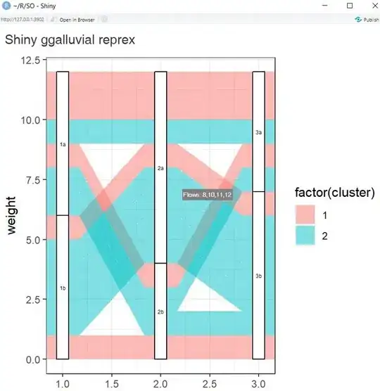
Hovering over a stratum
Code
library(tidyverse)
library(ggalluvial)
library(shiny)
library(sp)
library(htmltools)

### Function definitions
### ====================

# Slightly modified version of a function from ggalluvial
# Creates polygon coordinates from subset of built ggplot data
draw_by_group <- function(dat) {
  first_row <- dat[1, setdiff(names(dat),
                              c("x", "xmin", "xmax",
                                "width", "knot.pos",
                                "y", "ymin", "ymax")),
                   drop = FALSE]
  rownames(first_row) <- NULL

  curve_data <- ggalluvial:::data_to_xspline(dat, knot.prop = TRUE)
  data.frame(first_row, curve_data)
}


### Data
### ====

example_data <- data.frame(weight = rep(1, 12),
                           ID = 1:12,
                           cluster = c(rep(c(1,2), 5),2,2),
                           grp1 = rep(c('1a','1b'), c(6,6)),
                           grp2 = rep(c('2a','2b','2a'), c(3,4,5)),
                           grp3 = rep(c('3a','3b'), c(5,7)))
example_data <- example_data[order(example_data$cluster), ]

offset <- 5 # Maybe needed so that the tooltip doesn't disappear?

### UI function
### ===========

ui <- fluidPage(
  titlePanel("Shiny ggalluvial reprex"),
  fluidRow(tags$div(
    style = "position: relative;",
    plotOutput("sankey_plot", height = "800px",
               hover = hoverOpts(id = "plot_hover")),
    htmlOutput("tooltip")))
)

### Server function
### ===============

server <- function(input, output, session) {

  # Make and build plot.
  p <- ggplot(example_data, aes(y = weight, axis1 = grp1, axis2 = grp2, axis3 = grp3)) +
    geom_alluvium(aes(fill = factor(cluster)), knot.pos = 0) + # color for connections
    geom_stratum(width = 1/8, reverse = TRUE) + # plot the boxes over the connections
    geom_text(aes(label = after_stat(stratum)),
              stat = "stratum",
              reverse = TRUE,
              size = rel(1.5)) + # plot the text
    theme_bw() # black and white theme

  pbuilt <- ggplot_build(p)

  # Use built plot data to calculate the locations of the flow polygons
  data_draw <- transform(pbuilt$data[[1]], width = 1/3)

  groups_to_draw <- split(data_draw, data_draw$group)
  polygon_coords <- lapply(groups_to_draw, draw_by_group)

  output$sankey_plot <- renderPlot(p, res = 200)

  output$tooltip <- renderText(
    if(!is.null(input$plot_hover)) {
      hover <- input$plot_hover
      x_coord <- round(hover$x)

      if(abs(hover$x - x_coord) < 1/16) {
        # Display node information if mouse is over a node "box"
        box_labels <- c('grp1', 'grp2', 'grp3')
        # Determine stratum (node) name from x and y coord, and the n.
        node_row <- pbuilt$data[[2]]$x == x_coord & hover$y > pbuilt$data[[2]]$ymin & hover$y < pbuilt$data[[2]]$ymax
        node_label <- pbuilt$data[[2]]$stratum[node_row]
        node_n <- pbuilt$data[[2]]$n[node_row]
        renderTags(
          tags$div(
            "Category:", box_labels[x_coord], tags$br(),
            "Node:", node_label, tags$br(),
            "n =", node_n,
            style = paste0(
              "position: absolute; ",
              "top: ", hover$coords_css$y + offset, "px; ",
              "left: ", hover$coords_css$x + offset, "px; ",
              "background: gray; ",
              "padding: 3px; ",
              "color: white; "
            )
          )
        )$html
      } else {
        # Display flow information if mouse is over a flow polygon: what alluvia does it pass through?

        # Calculate whether coordinates of hovering mouse are inside one of the polygons.
        hover_within_flow <- sapply(polygon_coords, function(pol) point.in.polygon(point.x = hover$x, point.y = hover$y, pol.x = pol$x, pol.y = pol$y))
        if (any(hover_within_flow)) {
          # Find the alluvium that is plotted on top. (last)
          coord_id <- rev(which(hover_within_flow == 1))[1]
          # Get the corresponding row ID from the main data frame
          flow_id <- example_data$ID[coord_id]

          # Get the subset of data frame that has all the characteristics matching that alluvium
          data_row <- example_data[example_data$ID == flow_id, c('cluster', 'grp1', 'grp2', 'grp3')]
          IDs_show <- example_data$ID[apply(example_data[, c('cluster', 'grp1', 'grp2', 'grp3')], 1, function(x) all(x == data_row))]

          renderTags(
            tags$div(
              "Flows:", paste(IDs_show, collapse = ','),
              style = paste0(
                "position: absolute; ",
                "top: ", hover$coords_css$y + offset, "px; ",
                "left: ", hover$coords_css$x + offset, "px; ",
                "background: gray; ",
                "padding: 3px; ",
                "color: white; "
              )
            )
          )$html
        }
      }
    }
  )

}

shinyApp(ui = ui, server = server)
Additional explanation
This takes advantage of the built-in plot interaction in Shiny. By adding the argument hover = hoverOpts(id = "plot_hover") to plotOutput(), the input object now includes the coordinates of the hovering mouse in units of plot coordinates, making it very easy to locate where on the plot the mouse is.
The server function draws the ggalluvial plot and then manually recreates the boundaries of the polygons representing the alluvia. This is done by building the ggplot2 object and extracting the data element from it, then passing that to the unexported function from the ggalluvial source code (data_to_xspline). Next there is logic that detects whether the mouse is hovering over a node or a link, or neither. The nodes are easy since they are rectangles but whether the mouse is over a link is detected using sp::point.in.polygon(). If the mouse is over a link, all the row IDs from the input dataframe that match the characteristics of the selected link are extracted. Finally the tooltip is rendered with the function htmltools::renderTags().


