I am trying to plot a scatter graph onto my 3d continuous graph in python using matplotlib

Question

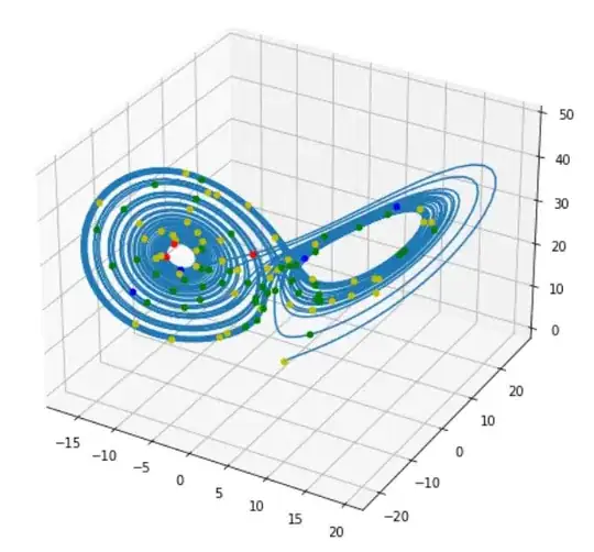
I have plotted the Lorenz attractor on a 3d graph. I am wanting to see how the size of the growth rates of the bred vectors affect the lorenz attractor, by plotting different coloured points representing different sizes of growth rates onto the lorenz graph.

This is the code I have at the moment:

fig = plt.figure(figsize=(8, 8))
ax = fig.add_subplot(111, projection = '3d')

plot lorenz

ax.plot(x1, y1, z1)

add growth rate markers

ax = fig.add_subplot

for k in range(100):
    if (GR[k] <= 0):
      plt.scatter(0.5*k, x1[50*k], c = "y")
    elif (0 < GR[k] <= 3.2):
      plt.scatter(0.5*k, x1[50*k], c = "g")
    elif (3.2 < GR[k] <= 6.4):
      plt.scatter(0.5*k, x1[50*k], c = "b")
    else:
      plt.scatter(0.5*k, x1[50*k], c = "r")

x1, y1, z1 make up the lorenz attractor, and GR is the growth rates of the bred vectors, the first 50 of which are:

  [0.          10.282047    10.8977816    9.94731134   5.09550477
  -2.90817325  -8.55789949 -10.22519406  -7.08646881  -4.03173251
   0.32302345   2.48287221  -0.64753007  -1.22328369   1.14720494
   0.50083297  -1.24334573  -1.97221857   1.48577796   2.20605109
  -1.09659768  -0.82320336   1.23992983   0.32689335  -1.35888724
  -1.8668327    1.79410769   1.84711434  -1.38602027  -0.44126068
   1.28436189   0.27735059  -1.35896733  -1.81959438   1.87149091
   1.53278532  -1.54682835  -0.15104558   1.35899661   0.39353056
  -1.21200428  -1.86788144   1.69061062   1.31533289  -1.6250634
   0.01201846   1.5258175    0.71428205  -0.86708544  -1.95685686]

At the line plt.scatter(0.5*k, x1[50*k], c = "y"), this error comes up:

TypeError: loop of ufunc does not support argument 0 of type NoneType which has no callable sqrt method

I have also attempted to plot the scatter graph this way:

ax = fig.add_subplot
for k in range(100):
    if (GR[k] <= 0):
      plt.scatter(0.5*k, x1[50*k], y1[50*k], z1[50*k], c = "y")
    elif (0 < GR[k] <= 3.2):
      plt.scatter(0.5*k, x1[50*k], y1[50*k], z1[50*k], c = "g")
    elif (3.2 < GR[k] <= 6.4):
      plt.scatter(0.5*k, x1[50*k], y1[50*k], z1[50*k], c = "b")
    else:
      plt.scatter(0.5*k, x1[50*k], y1[50*k], z1[50*k], c = "r")

But at the line plt.scatter(0.5*k, x1[50*k], y1[50*k], z1[50*k], c = "y") this comes up with the following error:

TypeError: scatter() got multiple values for argument 'c'

Can anyone help with this?

Below is an MIV that should be able to be run locally:

import numpy as np
from scipy.integrate import solve_ivp
import matplotlib.pyplot as plt

#Initial Conditions
X0 = np.array([1, 1, 1])

#define lorenz function
def lorenz_solveivp(sigma=10, r=28, b=8/3):
    def rhs(t, X):
        return np.array([sigma*(X[1] - X[0]), -X[0]*X[2] + r*X[0] - X[1], X[0]*X[1] - b*X[2]])
    return rhs

#define time and apply solve_ivp
t = np.linspace(0, 50, 5001)  #equispaced points from 0 to 50, timestep of 0.01
rhs_function = lorenz_solveivp()
sol1 = solve_ivp(rhs_function, (0, 50), X0, t_eval=t)

#find the growth rates
def growth_rate(X0, dX, n, dt, ng):
    Xp0 = X0 + dX
    times = np.linspace(0, n*dt, n + 1)
    Xn_save = np.zeros((X0.size, n*(ng-1)+1))
    Xpn_save = np.zeros((Xp0.size, n*(ng-1)+1))
    t = np.zeros((n*(ng - 1) + 1))
    i = 0
    g = np.zeros(ng)

    while i < ng - 1:

        Xn = solve_ivp(lorenz_solveivp(), [0, n*dt], X0, t_eval = times)
        Xpn = solve_ivp(lorenz_solveivp(), [0, n*dt], Xp0, t_eval = times)

        Xn_save[:, n*i: n + 1 + n*i] = Xn.y
        Xpn_save[:, n*i: n + 1 + n*i] = Xpn.y
        t[n*i: n + 1 + n*i] = Xn.t + i*n*dt

        dXb = Xpn.y[:,n] - Xn.y[:,n]

        g[i+1] = np.log(np.linalg.norm(dXb)/np.linalg.norm(dX))/(n*dt)

        P_new = dXb*(np.linalg.norm(dX)/np.linalg.norm(dXb))
        Xp0 = Xn.y[:,n] + P_new
        X0 = Xn.y[:,n]
        i += 1

    return g, Xn_save, t

X0 = np.array([1, 1, 1])
dX = np.array([1, 1, 1])/(np.sqrt(3))
dt = 0.01
n = 8
ng = 1000
GR, Xn_save, t = growth_rate(X0, dX, n, dt, ng)

#plot lorenz function
x1, y1, z1 = sol1.y

fig = plt.figure(figsize=(8, 8)) #specify the size of plot
ax = fig.add_subplot(111, projection = '3d')
ax.plot(x1, y1, z1)

# add growth rate markers
ax = fig.add_subplot
for k in range(100):
    if (GR[k] <= 0):
      plt.scatter(0.5*k, x1[50*k], y1[50*k], z1[50*k], color = "y")
    elif (0 < GR[k] <= 3.2):
      plt.scatter(0.5*k, x1[50*k], y1[50*k], z1[50*k], color = "g")
    elif (3.2 < GR[k] <= 6.4):
      plt.scatter(0.5*k, x1[50*k], y1[50*k], z1[50*k], color = "b")
    else:
      plt.scatter(0.5*k, x1[50*k], y1[50*k], z1[50*k], color = "r")

Please provide a [MIVE](https://stackoverflow.com/help/minimal-reproducible-example). And check the [matplotlib documentation](https://matplotlib.org/api/_as_gen/mpl_toolkits.mplot3d.axes3d.Axes3D.html) for how to make 3d plots (your scatters are missing z coordinates). It is not clear from your question where in your code the type error came from. — cvanelteren, Dec 22 '20 at 12:42
@cvanelteren thanks for answering. Sorry, I am unsure what an MIVE is. I have updated the question to make it clear where the error occurs. I have tried it with including y and z coordinates as well, but an error appear about multiple values for argument 'c' - I will edit the post again to what I tried and what happened. — USer555, Dec 22 '20 at 13:00
Checkout the [docs](https://matplotlib.org/3.3.3/api/_as_gen/matplotlib.pyplot.scatter.html) for scatter. The argument `c` needs to be an array. Change the code from `c` to `color =`. — cvanelteren, Dec 22 '20 at 13:16
In addition the `MIVE` is linked above. You question here is not a code I can run here locally without access to the data. — cvanelteren, Dec 22 '20 at 13:17
@cvanelteren thank you! I have now added in a MIV - apologies for not having this in earlier. I have also tried to chang 'c' to 'color' for the plots but it comes up with the following error: "ValueError: Supply a 'c' argument or a 'color' kwarg but not both; they differ but their functionalities overlap.". Which is very confusing because I have removed all the 'c' arguments. — USer555, Dec 22 '20 at 13:40

score 0 · Accepted Answer · answered Dec 23 '20 at 09:29

I fixed your code. There were 2 main problems with the code

By default matplotlib has 2D line plots plt.plot defaults to 2d. I fixed this by plotting directly on your 3d axis
removed 0.5 * k as I am not sure what this was doing but wasn't part of the 3d coordinate system I think.

import numpy as np
from scipy.integrate import solve_ivp
from mpl_toolkits.mplot3d import Axes3D
import matplotlib.pyplot as plt

#Initial Conditions
X0 = np.array([1, 1, 1])

#define lorenz function
def lorenz_solveivp(sigma=10, r=28, b=8/3):
    def rhs(t, X):
        return np.array([sigma*(X[1] - X[0]), -X[0]*X[2] + r*X[0] - X[1], X[0]*X[1] - b*X[2]])
    return rhs

#define time and apply solve_ivp
t = np.linspace(0, 50, 5001)  #equispaced points from 0 to 50, timestep of 0.01
rhs_function = lorenz_solveivp()
sol1 = solve_ivp(rhs_function, (0, 50), X0, t_eval=t)

#find the growth rates
def growth_rate(X0, dX, n, dt, ng):
    Xp0 = X0 + dX
    times = np.linspace(0, n*dt, n + 1)
    Xn_save = np.zeros((X0.size, n*(ng-1)+1))
    Xpn_save = np.zeros((Xp0.size, n*(ng-1)+1))
    t = np.zeros((n*(ng - 1) + 1))
    i = 0
    g = np.zeros(ng)

    while i < ng - 1:

        Xn = solve_ivp(lorenz_solveivp(), [0, n*dt], X0, t_eval = times)
        Xpn = solve_ivp(lorenz_solveivp(), [0, n*dt], Xp0, t_eval = times)

        Xn_save[:, n*i: n + 1 + n*i] = Xn.y
        Xpn_save[:, n*i: n + 1 + n*i] = Xpn.y
        t[n*i: n + 1 + n*i] = Xn.t + i*n*dt

        dXb = Xpn.y[:,n] - Xn.y[:,n]

        g[i+1] = np.log(np.linalg.norm(dXb)/np.linalg.norm(dX))/(n*dt)

        P_new = dXb*(np.linalg.norm(dX)/np.linalg.norm(dXb))
        Xp0 = Xn.y[:,n] + P_new
        X0 = Xn.y[:,n]
        i += 1

    return g, Xn_save, t

X0 = np.array([1, 1, 1])
dX = np.array([1, 1, 1])/(np.sqrt(3))
dt = 0.01
n = 8
ng = 1000
GR, Xn_save, t = growth_rate(X0, dX, n, dt, ng)

#plot lorenz function
x1, y1, z1 = sol1.y

fig = plt.figure(figsize=(8, 8)) #specify the size of plot
ax = fig.add_subplot(111, projection = '3d')
ax.plot(x1, y1, z1)

# add growth rate markers
for k in range(100):
    # simplified expression to set color
    if (GR[k] <= 0):
        c = 'y'
    elif (0 < GR[k] <= 3.2):
        c = 'g'
    elif (3.2 < GR[k] <= 6.4):
        c = 'b'
    else:
        c = 'r'
    ax.scatter(x1[50*k], y1[50*k], z1[50*k], color = c)
fig.show()

Thank you very much!!! this exactly what I was aiming for! – USer555 Dec 23 '20 at 13:43 — USer555, Dec 23 '20 at 13:43

I am trying to plot a scatter graph onto my 3d continuous graph in python using matplotlib

plot lorenz

add growth rate markers

1 Answers1