5

enter image description here

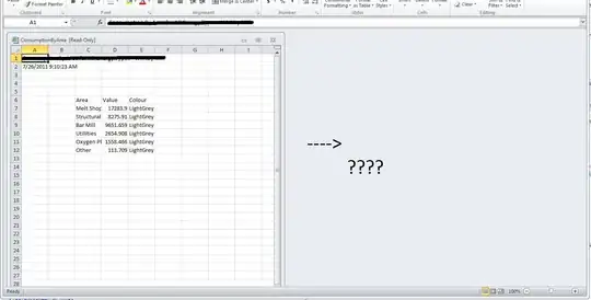
As shown in the 2 images, there are 2 sheets. "Result" is the sheets I want the result to be in and the "From" sheet is the source to search from. Basically, I want to search for the names of that student based on the "class number" and "student number". Neither "class number" nor "student number" is unique which means there are possible duplicates. However, the combination of "class number" and "student number" is unique, which means each student would have a different "class number" and "student number" combination. So the approach I thought was to first create a supporting column that concats "class number" and "student number" and then do a VlookUp. The code is as follow:

Sub vlookupName()
    
    'get the last row of both sheets
    resultRow = Sheets("Result").[a1].CurrentRegion.Rows.Count
    fromRow = Sheets("From").[a1].CurrentRegion.Rows.Count
    
    'concat Class number and student number to get a unique string used for vlookup
    Sheets("Result").Range("D2:D" & resultRow) = "=B2 & C2"
    Sheets("From").Columns("A").Insert
    Sheets("From").Range("A2:A" & resultRow) = "=c2 & d2"
    
    'vlookup
    Sheets("Result").Range("A2:A" & resultRow) = Application.VLookup(Sheets("Result").Range("D2:D" & resultRow).Value, _
        Sheets("From").Range("a2:b" & fromRow).Value, 2, False)
        
    '(delete columns to get back to raw file for next test)
    Sheets("Result").Columns("D").Delete
    Sheets("From").Columns("A").Delete
    Sheets("Result").Range("A2:A" & resultRow) = ""
End Sub

Improvements of any part of the code or methods are appreciated.

JackeyOL
  • 313
  • 2
  • 16
  • Instead of `=B2 & C2` you should be using a formula with a delimiter, such as (eg) `=B2 & "~" & C2` , otherwise (for example) 1 and 15 would match against 11 and 5 – Tim Williams Sep 02 '21 at 23:16
  • You are totally right, I missed that when making up this test file for illustrative purpose. In the real world problem, the two columns are of the same length, so this should be a problem. However, my code just couldn't find any result back and I'm super confused. @TimWilliams – JackeyOL Sep 02 '21 at 23:26
  • We can't see your data so it's difficult for us to offer any input as to why you might not be getting the results you expect. – Tim Williams Sep 02 '21 at 23:27
  • 1
    Reading your statement *"the combination of "class number" and "student number" is unique..."* I don't understand why there are two identical `class` - `student` combinations in your example, i.e. `5` and `13` (referring to *Bobby* and *Jayce*); is this just a typo in your example data? - @JackeyOL – T.M. Sep 06 '21 at 17:53
  • When using Excel365 use the FILTER-function, it's made for this. See answer of lke below – EvR Sep 09 '21 at 15:33
  • @T.M. thank you for pointing it out and that's just simply a typo when I created this example. – JackeyOL Sep 12 '21 at 03:19
  • Thank you for response; anyway I considered this case (as well as non-findings) in both of my approaches here @JackeyOL – T.M. Sep 12 '21 at 07:49

8 Answers8

8

Concatenating is dangerous when trying to lookup with multiple values. Consider the following 2 cases:

Class Number Student Number
1 15
11 5

Both concatenations will result in 115 and that's simply not unique.

You could argue that adding a delimiter could fix that. Something like an underscore and the 2 examples above would become 1_15 and 11_5. Yes, that would work as long as your parts are numeric but what if they were texts? Something like:

Part 1 Part 2
1_ 5
1 _5

Both concatenations will result in 1__5 and that's also not unique. Although this last example is forced I hope it proves the point that this approach is not clean and can lead to wrong results.

Based on the ranges shown in your 2 images, I would write the following formula in cell A2 of the Result sheet:

=INDEX(From!$A$2:$A$11,MATCH(1,INDEX((From!$B$2:$B$11=$B2)*(From!$C$2:$C$11=$C2),0),0))

or in a more english way:

=INDEX(ResultRange,MATCH(1,INDEX((KeyPart1Range=DesiredPart1)*(KeyPart2Range=DesiredPart2),0),0)) which can easily be extended by adding part3, part4 and so on to match as many criterias as needed.

The logic is simple:

  1. Something like From!$B$2:$B$11=$B2 will return an array of boolean values (TRUE and FALSE) corresponding to the number of rows in the From!$B$2:$B$11 range
  2. Multiplying two (or more) arrays of booleans will result in a single array of 1 and 0 where 1 means TRUE and 0 means FALSE
  3. The INDEX(array,0) will return the full array without the need to press Ctrl+Shift+Enter (needed for Excel versions that are not Office 365)
  4. The MATCH(1,...) will return the row index where all the specified criterias are met
  5. The outmost INDEX returns the desired result

Why would you want to run VBA code to recreate a formula that can be done directly in Excel? It ussually "smells" of bad practice. The maintainability of the whole project is made much more difficult by such an approach. If you rename sheets, you will need to update code. If you change the ranges (insert a column for example), you will need to update code. And the list goes on and on.

Assuming that you don't want formulas in your final result tab then why not just create an intermediate sheet that does all the formulas (Excel formulas) you want and then your code could simply do a copy-paste to the final result tab where there will be just values. This way if you need to add extra logic, you can just work on the intermediate sheet in plain Excel and not worry about synchronizing any code.

Cristian Buse
  • 4,020
  • 1
  • 13
  • 34
  • Thank you for the input. The reason I want a VBA solution is simply that it's just part of a large project for automating workflow and I'm using this artificial example purely for illustrative purposes. – JackeyOL Sep 12 '21 at 03:17
  • @JackeyOL Got it. Then you should be working with arrays directly in VBA without mixing with ranges especially if you're planning to read multiple external files. Power Query would be another alternative. I suggest you post a separate question on [Code Review](https://codereview.stackexchange.com/) outlining the whole workflow and what you've got so far so that you get reviews on the "architecture" of what you're trying to do. – Cristian Buse Sep 12 '21 at 06:20
4

Not a VBA answer as such but worth noting there's a "multi-column" version of MATCH() which could be used here:

enter image description here

Tim Williams
  • 154,628
  • 8
  • 97
  • 125
3

You can use the new FILTER-Function to retrieve the students name for a given class and student number. As the combination is unique the formula will return only one value.

In my example I assume that you use tables for the from-data and the result-data (Insert > Table). I prefer this method as you can use readable names within the formula.

enter image description here

=FILTER( tblData[Name], (tblData[Class Number]=[@[Class Number]])*(tblData[Student Number]=[@[Student Number]]), "[???]") will return

  • the students name (first parameter)
  • if class number and student number are matching --> two conditions "joined" by "multiplication" (second parameter).
  • In case there is no such combination [???] will be returned (third parameter)

If you want to keep the VBA-solution:

Public Sub lookupStudentName()
  Dim loResult As ListObject
  Set loResult = worksheet1.ListObjects("tblResult")

  loResult.ListColumns("Name").DataBodyRange.FormulaR1C1 = _
    "=FILTER(tblData[Name], _
     (tblData[Class Number]=[@[Class Number]])*(tblData[Student Number]=[@[Student Number]]), _
    ""[???]"")"
End Sub
Ike
  • 9,580
  • 4
  • 13
  • 29
1

If your dataset is small you may use an array and call it with an UDF. My FROM Sheet:

enter image description here

My RESULT sheet:

enter image description here

Code of my UDF:

Public Function GET_NAME(ByVal rng_data As Range, ByVal vStudent As Long, ByVal vClass As Long) As String
Application.Volatile
Dim MiMatriz As Variant
Dim i As Long

MiMatriz = rng_data.Value

For i = 1 To UBound(MiMatriz) Step 1
    If MiMatriz(i, 2) = vClass And MiMatriz(i, 3) = vStudent Then
        GET_NAME = MiMatriz(i, 1)
        Erase MiMatriz
        Exit Function
    End If
Next i

Erase MiMatriz
GET_NAME = "Not found"
End Function

I added a "not found" option in case there is no match.

The advantage of this method is that you don't need to worry about getting duplicates when joining student and class numbers.

But notice this will work properly if dataset is small. If it's too big, it may cause performance issues.

EDIT: I call this function typing =GET_NAME(From!$A$2:$C$8;Result!C2;Result!B2) in cell B2 and dragdown.

marc_s
  • 732,580
  • 175
  • 1,330
  • 1,459
1

If you dispose of MS Excel 365, it suffices to enter the following formula into cell A2 in sheet "Result", which displays all found names dynamically as a spill range; of course you can adapt the referring cell ranges to your needs.

=LET(Names,From!A2:A11,SrchId,TEXT(C2:C11+B2:B11*0.01,"0.00"),DataId,TEXT(From!C2:C11+From!B2:B11*0.01,"0.00"),INDEX(Names,MATCH(SrchId,DataId,0),1))

Explanation of the LET() function

LET enables you to

  • define expressions ("variables") together with their contents in pairs of arguments (i.e. a) Names referring to From!A2:A11, b) SrchId built from Result sheet, c) DataId based on sheet From) and

Methodical hint: Instead of concatenating Ids, this approach adds Student nums and class nums divided by 100 to a combined id.

  • let them follow a condensed last calculation part using the predefined expressions.

The calculation part as last argument of the LET function now simply reads as follows:

    INDEX(Names,MATCH(SrchId,DataId,0),1)

Benefits:

The formula architecture

  • improves performance as it avoids redundant, repeating calculations of identical references,
  • facilitates composition as it allows step to step assignments and
  • improves readibility, especially of the calculation part.

These points might meet to a certain degree the bountie's requirements of Elegance, effectiveness, and insightfulness.

T.M.
  • 9,436
  • 3
  • 33
  • 57
  • And what if the values are texts and not numbers? Multiplying with 0.01 is a trick, not an "elegant" solution and will return errors when dealing with text. What if the IDs are starting from 1 to 10000? Multiplying with 0.01 could return another valid ID isn't it? Like 10000 * 0.01 returns 100. The rest of the answer is nice but I warmly suggest you drop this kind of tricks. +1 – Cristian Buse Sep 07 '21 at 07:56
  • 1
    Appreciate your feedback touching indeed some important points to look at generally: - ad 1) Of course *mathematic* operations require a *coherent numeric* data base which, however should be assumed in OP. *I admit that this cannot be assumed in all cases.* - ad 2) Given a *case specific realistic limit* of classes of e.g. *~99 classes, the chosen multiplication by e.g. `0.01` is only executed upon the smaller part (►*class* data) , whereas the *student's id* can pass easily the number of 10000. The combined id thus remains unique. - @CristianBuse – T.M. Sep 07 '21 at 08:57
  • I totally agree it works in this specific situation. I was just saying it's a dangerous practice and should be avoided (before it develops into a habit and does damage somewhere else). Thanks for the extra explanation – Cristian Buse Sep 07 '21 at 09:12
  • 1
    I'd just say: Any find/match/Instr etc operation has its caveats. So coding always requires to know what you are doing which btw underlines the importance of a sufficient documentation. I do appreciate your pointing out a possible hurdle as it can contribute to a broader general understanding and may stimulate other code improvements. – T.M. Sep 10 '21 at 07:45
1

You don't need to use VBA for this but a couple of formulae will suffice.

In order to get Index to work well when matches aren't found you need to avoid 0 as a result from any calculation. One way to do this is to create an error when no match is found then trap it using IFERROR(value, value_if_error). Similarly a non-match when using MATCH will also give an error to be trapped.

So using a concatenation symbol to avoid spill you can get something like:

=IFERROR(INDEX(A$1:A$13,MATCH(I$1&"#"&J$1,B$1:B$13&"#"&C$1:C$13,0)),"")

You can also use SUMPRODUCT if you want (although there must uniqueness in the lookup data otherwise it would sum the multiple rows and give erroneous results from the INDEX):

=IFERROR(INDEX(A$1:A$13,SUMPRODUCT((B$1:B$13=I1)*(C$1:C$13=J1)*(ROW(B$1:B$13)))-ROW(B$1)+1),"")

Then if you want to reference a different worksheet, you would need to qualify each range with the respective worksheet reference, for example:

=IFERROR(INDEX(From!$A$2:$A$12,SUMPRODUCT((From!$B$2:$B$12=B2)*(From!$C$2:$C$12=C2)*(ROW(From!$B$2:$B$12)))-ROW(From!$B$2)+1),"")

Tragamor
  • 3,594
  • 3
  • 15
  • 32
1

You can try to use custom search function in sheet. And then use it as another built in function

Usage of custom function

Code of the function located at Module1 of the VBA in Excel sheet

Function SearchInTab(tabRange As range, classId As Integer, studentId As Integer)
    Dim tabRow As range
    For Each tabRow In tabRange.Rows
        Dim name As String
        Dim cls As Integer
        Dim std As Integer
        
        name = tabRow.Value2(1, 1)
        cls = tabRow.Value2(1, 2)
        std = tabRow.Value2(1, 3)
        
        If cls = classId And std = studentId Then
            SearchInTab = tabRow.Value2(1, 1)
            Exit Function
        End If
    Next
    SearchInTab = "NOT FOUND"
End Function

More about custom functions is HERE

Michael Navara
  • 1,111
  • 2
  • 8
  • 13
0

Alternative FilterXML approach

I'm demonstrating an alternative via FilterXML() function in three steps only:

  • a) define the data range - see help function getRange()
  • b) get student name(s) via FilterXML()
  • c) return the expected (unique) result (after an exceptions check for several or no findings)

Methodical hints

The FilterXML() function (available since vers. 2013+) requires the following arguments:

  • 1) a wellformed xml content string (roughly comparable to a html tags structure) - *see help function wellformed()*,
  • 2) a XPath expression defining here the searched node (i.e. <i>..</i>) at any hierarchy level //i as well as juxtaposed "And" conditions in brackets [..] defining the wanted value contents of the immediately following neighbour nodes.

Results in a string like <r><i>Amy</i><i>1</i><i>22</i><i>Richard</i><i>1</i><i>17</i>...</r> where the freely chosen name of <r> stands for the document element, i.e. root, <i> for item.

Further link @JvDV 's encyclopaedia like collection of FilterXML examples

Example of a user defined function GetStudentName()

Option Explicit                        ' declaration head of code module

Public Function GetStudentName(Class, StudentID) As String
'a) define full data range
    Dim DataRange As Range
    Set DataRange = GetRange(ThisWorkbook.Worksheets("From"))
'b) get student name(s) via FilterXML() based on wellformed content & XPath
    Dim tmp
    tmp = Application.FilterXML( _
        wellformed(DataRange), _
        "//i[following::*[1]='" & Class & "']" & _
        "[following::*[2]='" & StudentID & "']")
'c) return result string (after exceptions check for safety's sake)
    GetStudentName = check(tmp)
End Function

Help function wellformed()

The following help function builds a so-called "wellformed" xml string using the ►TextJoin() function available since versions 2019+. - It is easy, however to rewrite this function based on loops over all values in a datafield array based on the given range.

Function wellformed(rng As Range) As String
'Purp: return wellformed xml content string
'      (based on range input of several columns)
'Note: 1st argument of FilterXML() function

wellformed = "<r><i>" & WorksheetFunction.TEXTJOIN("</i><i>", True, rng) & "</i></r>"
End Function

Help function check()

Provides for possible exceptions (i.e. of 1 or several findings), as OP awaits only unique findings. Note that the late bound Application.FilterXML allows to analyze these exception without On Error handling.

Function check(tmp) As String
'Purp:  return Student Name as unique result and expected default, or
'       check exceptions zero or several findings (without On Error handling)
'a) provide for exceptions
    If TypeName(tmp) = "Variant()" Then ' found several elements
        tmp = UBound(tmp) & " elems: " & Join(Application.Transpose(tmp), ",")
    ElseIf IsError(tmp) Then            ' found no element at all
        tmp = "?"
    End If
'b) return function result
    check = tmp
End Function

Help function GetRange()

Simply returns the full data range of a referenced worksheet (here: "From"). Furthermore the function allows to define optional column boundaries, which might be used in other projects, too.

Function GetRange(ws As Worksheet, _
            Optional ByVal col = "A", _
            Optional ByVal col2 = "C", _
            Optional ByVal StartRow& = 2) As Range
'Purp: set full data range by calculation of last row in start column
'Note: assumes 3 columns range A:C by default (optional arguments)
'a) identify start and end column
    If IsNumeric(col) Then col = Split(ws.Cells(1, col).Address, "$")(1)
    If IsNumeric(col2) Then col2 = Split(ws.Cells(1, col2).Address, "$")(1)
'b) get last row in start column
    Dim LastRow As Long
    LastRow = ws.Range(col & Rows.Count).End(xlUp).Row
'c) return full range
    Set GetRange = ws.Range(col & StartRow & ":" & col2 & LastRow)
End Function
T.M.
  • 9,436
  • 3
  • 33
  • 57