How to plot a world map using R

Question

I am working on a project and a small part of it is plotting a world map with the 135 countries I have in my list. I also have a list that says whether they are developed or not.

How do I put this in the world map with different colors for the development status?

My data looks something like this

Country        Code      Developed
Brazil         BRA         1
Singapore      SIN         3
France         FRA         1
Poland         POL         2

I took the picture below from another question but ideally, it would look something like this but with more countries and 3 different colors.

Thanks

score 9 · Answer 1 · answered Oct 19 '21 at 06:04

First you need to install packages:

install.packages(c("cowplot", "googleway", "ggplot2", "ggrepel", 
"ggspatial", "libwgeom", "sf", "rnaturalearth", "rnaturalearthdata")

After that we gonna loading the basic packages necessary for all maps, i.e. ggplot2 and sf. We also suggest to use the classic dark-on-light theme for ggplot2 (theme_bw), which is appropriate for maps:

library("ggplot2")
theme_set(theme_bw())
library("sf")
library("rnaturalearth")
library("rnaturalearthdata")

world <- ne_countries(scale = "medium", returnclass = "sf")
class(world)

## [1] "sf"  
## [1] "data.frame"

After that we can:

ggplot(data = world) +
    geom_sf()

And the result gonna be like it:

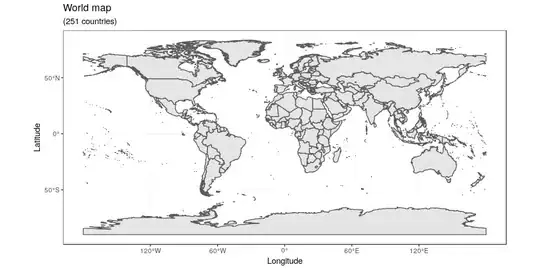
After it, we can add this:

ggplot(data = world) +
    geom_sf() +
    xlab("Longitude") + ylab("Latitude") +
    ggtitle("World map", subtitle = paste0("(", length(unique(world$NAME)), " countries)"))

and graph shows like this:

Finally, if we want some color, we need to do this:

ggplot(data = world) +
    geom_sf(aes(fill = pop_est)) +
    scale_fill_viridis_c(option = "plasma", trans = "sqrt")

This example shows the population of each country. In this example, we use the “viridis” colorblind-friendly palette for the color gradient (with option = "plasma" for the plasma variant), using the square root of the population (which is stored in the variable POP_EST of the world object)

You can learn more here:

https://r-spatial.org/r/2018/10/25/ggplot2-sf.html

https://datavizpyr.com/how-to-make-world-map-with-ggplot2-in-r/

https://slcladal.github.io/maps.html

Thanks. This teaches me how to draw up the map but not how to insert my data. — Rhedavetester, Oct 19 '21 at 06:23
@Rhedavetester you can use `left_join` to merge your data on the `sf` data of the world. Be careful with the country codes or name, have a look to `countrycode` package to normalize your country names — denis, Oct 19 '21 at 08:54

score 2 · Accepted Answer · answered Oct 19 '21 at 06:11

If you want to colour it with your own data, you will have to modify the world data frame accordingly:

library(rnaturalearth)
library(rnaturalearthdata)
library(ggplot2)
library(tidyverse)

world <- ne_countries(scale = "medium", returnclass = "sf")

my_countries <- c("Aruba","Afghanistan", "Morocco", "Canada")

world_modified <- world %>% 
  mutate(my_selection = ifelse(admin %in% my_countries,
                               1, NA))


ggplot(data = world_modified) +
  geom_sf(aes(fill=my_selection)) +
  theme_bw()

^{Created on 2021-10-19 by the reprex package (v2.0.0)}

How to plot a world map using R

2 Answers2