3

I am not sure if the title makes sense, but you can have a look at the example below. Considering I have a 2-column table in Excel like this:

Fruit   |   Amount
Apple   |     2
Grape   |     4
Orange  |     3

Now I want to have this row:

Apple | Apple | Grape | Grape | Grape | Grape | Orange | Orange | Orange

that when I change the number from "Amount" column in the table, the row changes accordingly as well. For example, if I now have 5 Grapes, it would become:

Apple | Apple | Grape | Grape | Grape | Grape | Grape | Orange | Orange | Orange

Is it possible to do in Excel? I am fairly new with this. Thanks!

Anthon1e
  • 45
  • 6

3 Answers3

4

Currently in BETA, but if available through insider's plan, try to use SCAN():

enter image description here

Formula in D1:

=XLOOKUP(SEQUENCE(1,SUM(B2:B4)),SCAN(0,B2:B4,LAMBDA(a,b,a+b)),A2:A4,,1)

Let me try and explain the steps:

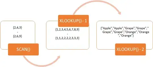
  • The SCAN() functionality can be used to create a running total. A starting value of 0 will continue to grow through recursive LAMBDA() functionality. In the current example this will return {2,6,9}.
  • Now the idea is to find approximate matches using XLOOKUP(). The input for this function is an array created through SEQUENCE() where the amount of columns will equal the SUM() of all amounts. Thus; {1,2,3,4,5,6,7,8,9} in this case. Using the 5th parameter we can return the position of the exact or nearest higher value in the lookup array we found using SCAN(). The result: {1,1,2,2,2,2,3,3,3}.
  • The next and last step is also done in XLOOKUP() where we used A2:A4 inside the 2nd parameter to return elements from the previous found numeric indices. Obviously the result will then be {"Apple","Apple","Grape","Grape","Grape","Grape","Orange","Orange","Orange"} .

I tried to visualize the above in a process that may help a little.

enter image description here


And as your amount change, so does the output as required:

enter image description here

JvdV
  • 70,606
  • 8
  • 39
  • 70
3

This can be achieved with a combination of

  • REPT - to generate the repated copies of the words
  • CONCAT - to join those repitions together
  • FILTERXML - to split the list into cells
  • TRANSPOSE - to return a row rather than a column
=TRANSPOSE(FILTERXML("<a>"&CONCAT("<b>"&REPT(B5:B7&"</b><b>",C5:C7-1)&B5:B7&"</b>")&"</a>","//b"))

enter image description here

chris neilsen
  • 52,446
  • 10
  • 84
  • 123
0

Here is a simple function to do a text multiple. You can then stack up the results.

Function TextMultiplier(MyText As String, MyMultiple As Integer)

Dim Output As String

For a = 1 To MyMultiple
    Output = Output + MyText + " "
Next a

TextMultiplier = Trim(Output)

End Function

Here is how it looks:

enter image description here

Jeremy Caney
  • 7,102
  • 69
  • 48
  • 77
Andy C
  • 11