Can this integral be done numerically in either Matlab or Mathematica?

Question

I want to be able to do the integral below completely numerically.

where 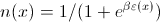, and , and are constants which for simplicity, can all be set to 1.

The integral over x can be done analytically by hand or using Mathematica, and then the integral over y can be done numerically using NIntegrate, but these two methods give different answers.

Analytically:

In[160]:= ex := 2 (1 - Cos[x])

In[149]:= ey := 2 (1 - Cos[y])

In[161]:= kx := 1/(1 + Exp[ex])

In[151]:= ky := 1/(1 + Exp[ey])

In[162]:= Fn1 := 1/(2 \[Pi]) ((Cos[(x + y)/2])^2)/(ex - ey)

In[163]:= Integrate[Fn1, {x, -Pi, Pi}]

Out[163]= -(1/(4 \[Pi]))
 If[Re[y] >= \[Pi] || \[Pi] + Re[y] <= 0 || 
   y \[NotElement] Reals, \[Pi] Cos[y] - Log[-Cos[y/2]] Sin[y] + 
   Log[Cos[y/2]] Sin[y], 
  Integrate[Cos[(x + y)/2]^2/(Cos[x] - Cos[y]), {x, -\[Pi], \[Pi]}, 
   Assumptions -> ! (Re[y] >= \[Pi] || \[Pi] + Re[y] <= 0 || 
       y \[NotElement] Reals)]]

In[164]:= Fn2 := -1/(
  4 \[Pi]) ((\[Pi] Cos[y] - Log[-Cos[y/2]] Sin[y] + 
     Log[Cos[y/2]] Sin[y]) (1 - ky) ky )/(2 \[Pi])

In[165]:= NIntegrate[Fn2, {y, -Pi, Pi}]

Out[165]= -0.0160323 - 2.23302*10^-15 I

Numerical method 1:

In[107]:= Fn4 := 
 1/(4 \[Pi]^2) ((Cos[(x + y)/2])^2) (1 - ky) ky/(ex - ey)

In[109]:= NIntegrate[Fn4, {x, -Pi, Pi}, {y, -Pi, Pi}]

During evaluation of In[109]:= NIntegrate::slwcon: Numerical integration converging too slowly; suspect one of the following: singularity, value of the integration is 0, highly oscillatory integrand, or WorkingPrecision too small. >>

During evaluation of In[109]:= NIntegrate::ncvb: NIntegrate failed to converge to prescribed accuracy after 18 recursive bisections in x near {x,y} = {0.0000202323,2.16219}. NIntegrate obtained 132827.66472461013` and 19442.543606302774` for the integral and error estimates. >>

Out[109]= 132828.

Numerical 2:

In[113]:= delta = .001;
pw[x_, y_] := Piecewise[{{1, Abs[Abs[x] - Abs[y]] > delta}}, 0]

In[116]:= Fn5 := (Fn4)*pw[Cos[x], Cos[y]]

In[131]:= NIntegrate[Fn5, {x, -Pi, Pi}, {y, -Pi, Pi}]

During evaluation of In[131]:= NIntegrate::slwcon: Numerical integration converging too slowly; suspect one of the following: singularity, value of the integration is 0, highly oscillatory integrand, or WorkingPrecision too small. >>

During evaluation of In[131]:= NIntegrate::eincr: The global error of the strategy GlobalAdaptive has increased more than 2000 times. The global error is expected to decrease monotonically after a number of integrand evaluations. Suspect one of the following: the working precision is insufficient for the specified precision goal; the integrand is highly oscillatory or it is not a (piecewise) smooth function; or the true value of the integral is 0. Increasing the value of the GlobalAdaptive option MaxErrorIncreases might lead to a convergent numerical integration. NIntegrate obtained 0.013006903336304906` and 0.0006852739534086272` for the integral and error estimates. >>

Out[131]= 0.0130069

So neither of the numerical methods give -0.0160323. I understand why - the first method has trouble with the infinities caused by the denominator, and the second method effectively deletes the part of the integral that is causing problems. But I'd like to be able to integrate another integral (a harder one over x, y and z) which can't be simplified analytically. The above integral gives me a way to test any new method since I know what the answer should be.

Answer 1

Unless I wrote down the integral wrong, this should do the job:

n[x_] := 1/(1 + Exp[eps[x]])
eps[x_] := 2(1 - Cos[x])
.25/(2*Pi)^2*NIntegrate[
    Cos[(x + y)/
     2]^2 ((1 - n[y]) n[y] - (1 - n[x]) n[x])/(Cos[y] - Cos[x]),
    {x, -Pi, Pi},
    {y, -Pi, Pi},
    Exclusions -> {Cos[x] == Cos[y]}
  ]

giving 0.0130098.

OK, I guess the quickest way to explain is like this:

going from the first to the second line of the first eq I've just renamed y to x (the region of integration is symmetric so it's OK). Then I have added the two (equivalent) expressions for I to obtain 2I, and what I numerically integrate is that. The point is that the numerator and denominator vanish at the same points, so in fact the Exclusions option isn't needed. Note that in my sketch of the method above I dropped the 1/(4*Pi^2) for brevity (or due to laziness, depending on the viewpoint).