Definition lookup speed: a performance issue

Question

I have the following problem.

I need to build a very large number of definitions(*) such as

f[{1,0,0,0}] = 1
f[{0,1,0,0}] = 2
f[{0,0,1,0}] = 3
f[{0,0,0,1}] = 2
...
f[{2,3,1,2}] = 4
...
f[{n1,n2,n3,n4}] = some integer
...

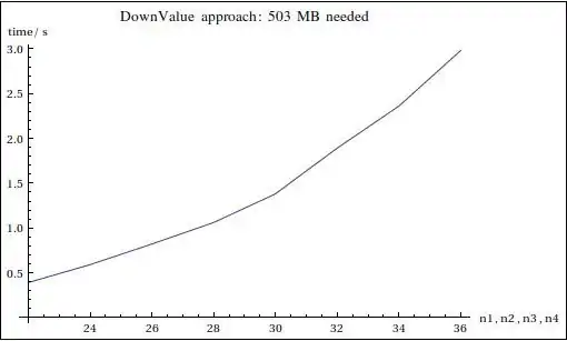
This is just an example. The length of the argument list does not need to be 4 but can be anything. I realized that the lookup for each value slows down with exponential complexity when the length of the argument list increases. Perhaps this is not so strange, since it is clear that in principle there is a combinatorial explosion in how many definitions Mathematica needs to store.

Though, I have expected Mathematica to be smart and that value extract should be constant time complexity. Apparently it is not.

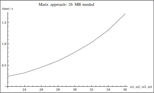
Is there any way to speed up lookup time? This probably has to do with how Mathematica internally handles symbol definition lookups. Does it phrases the list until it finds the match? It seems that it does so.

All suggestions highly appreciated. With best regards Zoran

(*) I am working on a stochastic simulation software that generates all configurations of a system and needs to store how many times each configuration occurred. In that sense a list {n1, n2, ..., nT} describes a particular configuration of the system saying that there are n1 particles of type 1, n2 particles of type 2, ..., nT particles of type T. There can be exponentially many such configurations.

Answer 1

Could you give some detail on how you worked out that lookup time is exponential?

If it is indeed exponential, perhaps you could speed things up by using Hash on your keys (configurations), then storing key-value pairs in a list like {{key1,value1},{key2,value2}}, kept sorted by key and then using binary search (which should be log time). This should be very quick to code up but not optimum in terms of speed.

If that's not fast enough, one could think about setting up a proper hashtable implementation (which I thought was what the f[{0,1,0,1}]=3 approach did, without having checked).

But some toy example of the slowdown would be useful to proceed further...

EDIT: I just tried

test[length_] := Block[{f},
  Do[
   f[RandomInteger[{0, 10}, 100]] = RandomInteger[0, 10];,
   {i, 1, length}
   ];
  f[{0, 0, 0, 0, 1, 7, 0, 3, 7, 8, 0, 4, 5, 8, 0, 8, 6, 7, 7, 0, 1, 6,
      3, 9, 6, 9, 2, 7, 2, 8, 1, 1, 8, 4, 0, 5, 2, 9, 9, 10, 6, 3, 6, 
     8, 10, 0, 7, 1, 2, 8, 4, 4, 9, 5, 1, 10, 4, 1, 1, 3, 0, 3, 6, 5, 
     4, 0, 9, 5, 4, 6, 9, 6, 10, 6, 2, 4, 9, 2, 9, 8, 10, 0, 8, 4, 9, 
     5, 5, 9, 7, 2, 7, 4, 0, 2, 0, 10, 2, 4, 10, 1}] // timeIt
  ]

with timeIt defined to accurately time even short runs as follows:

timeIt::usage = "timeIt[expr] gives the time taken to execute expr,
  repeating as many times as necessary to achieve a total time of \
1s";

SetAttributes[timeIt, HoldAll]
timeIt[expr_] := Module[{t = Timing[expr;][[1]], tries = 1},
    While[t < 1.,
    tries *= 2;
    t = Timing[Do[expr, {tries}];][[1]];
    ];
    Return[t/tries]]

and then

out = {#, test[#]} & /@ {10, 100, 1000, 10000, 100000, 100000};
ListLogLogPlot@out

(also for larger runs). So it seems constant time here.

Answer 2

Suppose you enter your information not like

f[{1,0,0,0}] = 1
f[{0,1,0,0}] = 2

but into a n1 x n2 x n3 x n4 matrix m like

m[[2,1,1,1]] = 1
m[[1,2,1,1]] = 2

etc.

(you could even enter values not as f[{1,0,0,0}]=1, but as f[{1,0,0,0},1] with

  f[li_List, i_Integer] := Part[m, Apply[Sequence, li + 1]] = i;
  f[li_List] := Part[m, Apply[Sequence, li + 1]];

where you have to initialize m e.g. by m = ConstantArray[0, {4, 4, 4, 4}];)

Let's compare timings:

testf[z_] := 
  (
   Do[ f[{n1, n2, n3, n4}] = RandomInteger[{1,100}], {n1,z}, {n2,z}, {n3,z},{n4,z}];
   First[ Timing[ Do[ f[{n2, n4, n1, n3}], {n1, z}, {n2, z}, {n3, z}, {n4, z} ] ] ]
  ); 
Framed[
   ListLinePlot[
       Table[{z, testf[z]}, {z, 22, 36, 2}], 
       PlotLabel -> Row[{"DownValue approach: ", 
                          Round[MemoryInUse[]/1024.^2], 
                          " MB needed"
                         }], 
       AxesLabel -> {"n1,n2,n3,n4", "time/s"},ImageSize -> 500
   ]
]
Clear[f]; 
testf2[z_] := 
  (
    m = RandomInteger[{1, 100}, {z, z, z, z}]; 
    f2[ni__Integer] := m[[Sequence @@ ({ni} + 1)]]; 
    First[ Timing[ Do[ f2[{n2, n4, n1, n3}], {n1, z}, {n2, z}, {n3, z}, {n4, z}] ] ]
  )
Framed[
   ListLinePlot[
       Table[{z, testf2[z]}, {z, 22, 36, 2}], 
       PlotLabel -> Row[{"Matrix approach: ", 
                         Round[MemoryInUse[]/1024.^2], 
                         " MB needed"
                        }], 
       AxesLabel -> {"n1,n2,n3,n4", "time/s"}, ImageSize -> 500
  ]
]

gives

So for larger sets up information a matrix approach seems clearly preferrable.

Of course, if you have truly large data, say more GB than you have RAM, then you just have to use a database and DatabaseLink.