Improving positioning of map / polygon labels

Question

This is an extension to Improve centering county names ggplot & maps and ggplot centered names on a map. It is not only a theoretical problem, I came across that particular case on answering How merge specific states together by group with one label in ggplot2 in R?. Here, I found that there is an L-shaped "grid" which led to a midpoint position outside the polygon. Also, see Henrik's linked thread Calculate Centroid WITHIN / INSIDE a SpatialPolygon. .

I wondered if there might be ways to force the label into the polygon, for a "more intuitive" midpoint. "Intuitively" means probably "the point inside the polygon furthest away from any boundary" (an answer to a related thread suggested a function to calculate this, but this function doesn't seem to give a different result than rgeos::gCentroid in my example).

Any suggestion should be fully automated, ideally be applicable to any (ir-)regular polygon and also be independent on the coordinate projection (i.e., the coordinates aspect ratio should not matter) correction: Ideally it should depend on the coordinate projection, as this might move the text to an awkward position to the border. Thus, the ideal solution should probably calculate the label position at drawing time.

Very related would be https://gis.stackexchange.com/questions/29278/finding-point-in-country-furthest-from-boundary and https://mathoverflow.net/questions/161494/get-a-point-in-polygon-maximize-the-distance-from-borders, but I have no clue how to implement this in R / grid / ggplot2.

suppressMessages({library(ggh4x)
library(sf)
library(dplyr)
library(patchwork)
})

poly_foo <- data.frame(x = c(0:1, rep(2,4), rep(1.5,3), 0), y = c(rep(0,3), 1:3, 3:1, 1))

p <-  ggplot(poly_foo, aes(x, y) ) +
  geom_polygon(color = "black", fill = NA)
p1 <- p +
  stat_midpoint(aes(label = "ggh4x::stat_midpoint\nNot ideal"), geom = "text") 

## Convert to simple feature object for geom_sf
point_sf <- st_as_sf(poly_foo,  coords = c("x", "y"))
poly_sf <- 
  point_sf %>%
  summarise(geometry = st_combine(geometry)) %>%
  st_cast("POLYGON") %>%
  mutate(label = "sf::st_point_on_surface\nNot ideal")

p2 <- ggplot(poly_sf) +
  geom_sf() +
  geom_sf_text(aes(label = label))

## convert to spatial object (sp) for rgeos::gCentroid
xy_lab <- rgeos::gCentroid(as_Spatial(poly_sf))@coords
p3 <- ggplot(poly_sf) +
  geom_sf() +
  annotate(geom = "text", label = "rgeos::gCentroid\nNot ideal", 
           x = xy_lab[1], y = xy_lab[2])
p4 <- p  +
  annotate(geom = "text", x = 1.7, y = .5, label = "more\nintuitive\n\'midpoint\'") 
## it should ideally change with different coordinates
p5 <- p + coord_fixed() + 
  annotate(geom = "text", x = 1, y = .5, label = "more\nintuitive\n\'midpoint\'\ncoordinates changed")

p1 + p2 + p3 + plot_annotation(title = "Example problem")

## Desired output
p4 + p5 + plot_annotation(title = "Desired behaviour")

^{Created on 2022-06-26 by the reprex package (v2.0.1)}

Answer 1

You can use rgeos::polygonsLabel which computes optimal positions for placing labels inside polygons. The default method is "maxdist" which "tries to find the label position with a maximal distance from the polygon edges". Please note that rgeos will retire by the end of 2023.

library(rgeos)
library(sp)
poly_foo <- data.frame(x = c(0:1, rep(2,4), rep(1.5,3), 0), y = c(rep(0,3), 1:3, 3:1, 1))
xy.sp = SpatialPolygons(list(Polygons(list(Polygon(poly_foo)), ID = "test")))
plot(xy.sp)

polygonsLabel(xy.sp, "MY TEST LABEL")

plot(xy.sp)
polygonsLabel(xy.sp, "L\na\nb\ne\nl")

plot(xy.sp)
polygonsLabel(xy.sp, "MY TEST LABEL\n\n TWO LINES HIGH")

ggplot2 method

Store the labels in a vector (or in a column of your spatial data). Calculate the positions of the labels first, and then use these coordinates to plot a geom_text()-layer with the labels.

library(sf)
library(ggplot2)
# create your vector with labels here...
my.labels <- "This is a test\nlabel"
# I get an error when no plot is present before calculating the 
# label's coordinates.. so plot first, then discard
plot(xy.sp)
# calculate positions for labels
#   For the best results, make sure text height in the ggplot
#   matches the text-height when the positions are calculated !
#   Fiddle with the cex-argument in rgeos::polygonsLabels()
label.pos <- data.frame(
  polygonsLabel(xy.sp, my.labels, doPlot = FALSE),
  labelText = my.labels)
# ggplot polygon + label
ggplot() + 
  geom_sf(data = sf::st_as_sf(xy.sp)) +
  geom_text(data = label.pos, aes(x = X1, y = X2, label = labelText))

Answer 2

Using what you've got along with the information that @Henrik provided, this works pretty well.

There is a catch, though. ggplot text to plot sizing is not scaled uniformly. Are you using this in the viewer pane? Are you exporting this? What sizes are you using? For example, the title might be a font size of 15 at 300 dpi, but if you wanted to add text of the same size, you would have to set the size to 15/.pt (where .pt is a static value from the package ggplot2).

Additionally, the default font type in ggplot is not monospaced—every letter doesn't get the same amount of real estate (like courier, for example).

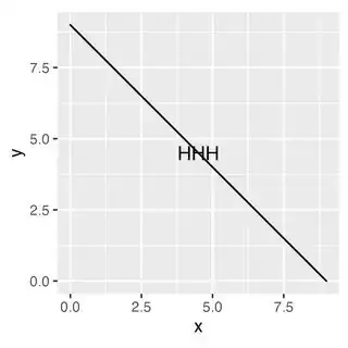
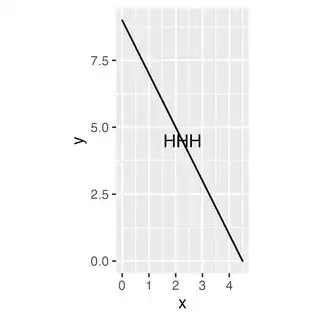
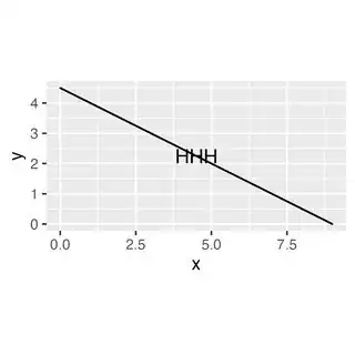
Check out these plots which have been saved at 300dpi, 3in x 3in, with the text size = 12/.pt and coord_equal. In the first plot "HHH" takes just over .25 units on the x-axis. In the second, it takes 1.5 units. In the last plot, it takes just over 1/2 unit.

This works. However, without a set scaling mechanism, it still requires manual intervention regarding either the font size or the string wrapping.

library(polylabelr)
library(stringr)
library(tidyverse)

poly_foo <- data.frame(x = c(0:1, rep(2,4), rep(1.5,3), 0),
                       y = c(rep(0,3), 1:3, 3:1, 1))

p <-  ggplot(poly_foo, aes(x, y) ) +
  geom_polygon(color = "black", fill = NA)
plr <- poi(poly_foo, precision, = .1)
p + 
  coord_equal() +
  annotate("text", x = plr$x, y = plr$y, label = "How about here?" %>% 
             str_wrap(., width = 9/(plr$dist * 2)))

pf2 <- mutate(poly_foo, x = x * 2, y = y^2)
poi2 <- poi(pf2, precision = .1)
ggplot(pf2, aes(x, y) ) +
  geom_polygon(color = "black", fill = NA) + 
  coord_equal() + 
  annotate("text", x = poi2$x, y = poi2$y,
           label = "Intuitive enough?" %>% 
             str_wrap(., width = 9/(poi2$dist * 2)))

pf3 <- mutate(poly_foo, x = x^2, y = y + 4)
poi3 <- poi(pf3, precision = .1)
ggplot(pf3, aes(x, y) ) +
  geom_polygon(color = "black", fill = NA) + 
  coord_equal() + 
  annotate("text", x = poi3$x, y = poi3$y, 
           label = "Intuitive enough?" %>% 
             str_wrap(., width = 9/(poi3$dist * 2)))

pf4 <- mutate(poly_foo, x = x^1/2, y = y^(1/3))
poi4 <- poi(pf4, precision = .1)
ggplot(pf4, aes(x, y) ) +
  geom_polygon(color = "black", fill = NA) + 
  coord_fixed() + 
  annotate("text", x = poi4$x, y = poi4$y,
           label = "Intuitive enough?" %>% 
             str_wrap(., width = 9/(poi4$dist * 2)))

Answer 3

Focusing on the calculated nature of the desired result, as applied to possibly 'annoying' label placement in polygons rather than label placement in arbitrary polygons, the following perhaps sketches an approach:

library(sf)
library(sfdct)
library(dplyr)
pf1 <- data.frame(x = c(0:1, rep(2,4), rep(1.5,3), 0),
                       y = c(rep(0,3), 1:3, 3:1, 1))

pf1_pt <- st_as_sf(x= pf1, coords=c('x', 'y'))

pf1_poly <- 
pf1_pt %>%
summarise(geometry = st_combine(geometry)) %>%
st_cast('POLYGON') %>%
mutate(label = 'Can be Very Long\nBut Informative!')

pt1_poly_tri <- st_cast(ct_triangulate(pf1_poly))
area_tri_pt1 <- as.numeric(st_area(pt1_poly_tri$geometry))

# get the largest triangles
pt1_poly_lbl_area <- st_union(pt1_poly_tri[area_tri_pt1 >= quantile(area_tri_pt1, 0.75), ])

# get a little more contiguous area, return centroid for ggplot label x,y

plot_lbl_xy <- st_coordinates(st_centroid(st_union(pt1_poly_lbl_area, pt1_poly_tri$geometry[[st_touches(pt1_poly_lbl_area, pt1_poly_tri)[[1]][2]]])))
plot_lbl_xy
  X   Y
1 1 0.5

I'll examine this in presence of holes shortly, or before deadline, hopefully. The difference between polygons without holes and polygons with holes, as triangulated via sfdct::ct_triangulate, is that in the first instance, without holes, one can receive a vector of return values of areas, whereas, in the presence of holes, at least for me, a loop is employed to secure individual triangle area values. Absent a loop, all values are summary (ie. total area under st_area) that is not desired.

The question, 'what are we dealing with here' can be addressed by st_is, where 'geometrycolledtion' will be TRUE in the case of holes present, FALSE otherwise.

The above sketch of approach where there are holes will fail; but, introducing a loop will work. Considering the following system of polygons:

outer2 <- matrix(c(0,0,0,32,4,32,4,17,11,17,11,29,15,29,15,17,22,11,22,31,24,31,24,18,29,18,36,12,24,0,0,0),ncol=2, byrow=TRUE)
hole1 <- matrix(c(7,14,7,15,6,15,6,15,7,14), ncol=2, byrow= TRUE)
hole2 <- matrix(c(2,3,7,3,7,5,2,3,2,3), ncol = 2, byrow = TRUE)
hole3 <- matrix(c(19,4, 21,6,17,10,15,8,19.4), ncol=2, byrow=TRUE)
my_painful_poly <- st_polygon(list(outer2,hole1,hole2,hole3))

a_label ='Muchos años después,\n frente al pelotón de fusilamiento,\n el coronel Aureliano Buendía\n había de recordar\n aquella tarde remota\n en que su padre\n lo llevó a conocer\n el hielo'

painful_ct <- ct_triangulate(my_painful_poly)
painful_area <- vector(mode = 'numeric', length=sum(lengths(painful_ct)))
for (m in 1:sum(lengths(painful_ct))) {
    painful_area[m] <- st_area(painful_ct[[m]])
  }
painful_area
 [1] 11.0  7.5  8.0 16.0 36.0 24.0 22.5 36.0 30.0 64.0  2.0 24.0  7.0  1.0  8.0
[16] 26.0 14.0 34.5  9.0 54.0 12.0 26.5 18.5 24.0 17.5 20.0 13.0 45.5 13.0

And so, we can proceed as above.

painful_lengths <- lengths(painful_ct)
which(seq(min(as.numeric(names(painful_lengths))), max(as.numeric(names(painful_lengths))), 1) %in% as.numeric(names(painful_lengths)) == FALSE)
[1]  5 10 18 20 # our holes as to plot order presumably

which seems analogous to @mdsomner 's reflections in sf-closed #693, whom also scripted the above in the context of a different problem mdsomner - finite element analysis as to quantile. But generally, the blame is mine.