What is the best practice to apply cross-validation using TimeSeriesSplit() over dataframe within end-2-end pipeline in python?

Question

Let's say I have dataset within the following pandas dataframe format with a non-standard timestamp column without datetime format as follows:

+--------+-----+
|TS_24hrs|count|
+--------+-----+
|0       |157  |
|1       |334  |
|2       |176  |
|3       |86   |
|4       |89   |
 ...      ...
|270     |192  |
|271     |196  |
|270     |251  |
|273     |138  |
+--------+-----+
274 rows × 2 columns

I have already applied some regression algorithms after splitting data without using cross-validation (CV) into training-set and test-set and got results like the following:

import numpy as np
import pandas as pd
import matplotlib.pyplot as plt

#Load the time-series data as dataframe
df = pd.read_csv('/content/U2996_24hrs_.csv', sep=",")
print(df.shape)

# Split the data into training and testing sets
from sklearn.model_selection import train_test_split
train, test = train_test_split(df, test_size=0.27, shuffle=False)
print(train.shape) #(200, 2)
print(test.shape)  #(74, 2)

#visulize splitted data
train['count'].plot(label='Training-set')
test['count'].plot(label='Test-set')
plt.legend()
plt.show()

#Train and fit the model
from sklearn.ensemble import RandomForestRegressor
rf = RandomForestRegressor().fit(train, train['count']) #X, y
rf.score(train, train['count']) #0.9998644192184375

# Use the forest's model to predict on the test-set
predictions = rf.predict(test)

#convert prediction result into dataframe for plot issue in ease
df_pre = pd.DataFrame({'TS_24hrs':test['TS_24hrs'], 'count_prediction':predictions})

# Calculate the mean absolute errors
from sklearn.metrics import mean_absolute_error
rf_mae = mean_absolute_error(test['count'], df_pre['count_prediction'])

print(train.shape)   #(200, 2)
print(test.shape)    #(74, 2)
print(df_pre.shape)  #(74, 2)

#visulize forecast or prediction of used regressor model
train['count'].plot(label='Training-set')
test['count'].plot(label='Test-set')
df_pre['count_prediction'].plot(label=f'RF_forecast  MAE={rf_mae:.2f}')
plt.legend()
plt.show()

According this answer I noticed:

if your data is already sorted based on time then simply use shuffle=False in train, test = train_test_split(newdf, test_size=0.3, shuffle=False)

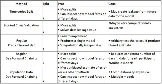
So far, I have used this classic split data method, but I want to experiment with Time-series-based split methods that are summarized here:

Additionally, based on my investigation (please see the references at the end of the post), it is recommended to use the cross-validation method (K-Fold) before applying regression models. explanation: Cross Validation in Time Series

Problem: How can split time-series data with using CV methods for comparable results? (plot the quality of data split for ensure\evaluate the quality of data splitting)

TSS CV method: TimeSeriesSplit()
BTSS CV method: BlockingTimeSeriesSplit()

So far, the closest solution that crossed my mind is to separate the last 74 observations as hold-on test-set a side and do CV on just the first 200 observations. I'm still struggling with playing with these arguments max_train_size=199, test_size=73 to reach desired results, but it's very tricky and I couldn't figure it out. in fact, I applied time-series-based data split using TSS CV methods before training RF regressor to train-set (first 200 days\observations) and fit model over test-set (last 74 days\observations).

I've tried recommended TimeSeriesSplit() as the following unsuccessfully:

import numpy as np
import pandas as pd
import matplotlib.pyplot as plt

#Load the time-series data as dataframe
df = pd.read_csv('/content/U2996_24hrs_.csv', sep=",")
print(df.shape)

#Try to split data with CV (K-Fold) by using TimeSeriesSplit() method
from sklearn.model_selection import TimeSeriesSplit
tscv = TimeSeriesSplit(
    n_splits=len(df['TS_24hrs'].unique()) - 1,
    gap=0, # since data alraedy groupedby for 24hours to retrieve daily count there is no need to to have gap
    #max_train_size=199, #here: https://stackoverflow.com/a/43326651/10452700 they recommended to set this argument I'm unsure if it is the case for my problem
    #test_size=73,
)

for train_idx, test_idx in tscv.split(df['TS_24hrs']):
    print('TRAIN: ',    df.loc[df.index.isin(train_idx), 'TS_24hrs'].unique(), 
          'val-TEST: ', df.loc[df.index.isin(test_idx),  'TS_24hrs'].unique())

The following figures for understanding and better alignment of split data could be part of the expected output if one could plot for each method:

expected output:

References:

Edit1:

I found 3 related posts:

post1
post2

I decided to apply TimeSeriesSplit() in short TTS cv output within for loop to train\fit regression model over training-set with assist of CV-set then predict() over Hold-on test-set. The current output of my implementation shows slightly improvement in forecasting with or without, which could be due to problems in my implementation.

#Load the time-series data as dataframe
import numpy as np
import pandas as pd
import matplotlib.pyplot as plt

df = pd.read_csv('/content/U2996_24hrs_.csv', sep=",")
#print(df.shape) #(274, 2)

#####----------------------------without CV

# Split the data into training and testing sets
from sklearn.model_selection import train_test_split
train, test = train_test_split(df, test_size=0.27, shuffle=False)
print(train.shape) #(200, 2)
print(test.shape)  #(74, 2)

#visulize splitted data
#train['count'].plot(label='Training-set')
#test['count'].plot(label='Test-set')
#plt.legend()
#plt.show()

#Train and fit the model
from sklearn.ensemble import RandomForestRegressor
rf = RandomForestRegressor().fit(train, train['count']) #X, y
rf.score(train, train['count']) #0.9998644192184375

# Use the forest's model to predict on the test-set
predictions = rf.predict(test)

#convert prediction result into dataframe for plot issue in ease
df_pre = pd.DataFrame({'TS_24hrs':test['TS_24hrs'], 'count_prediction':predictions})

# Calculate the mean absolute errors
from sklearn.metrics import mean_absolute_error
rf_mae = mean_absolute_error(test['count'], df_pre['count_prediction'])

#####----------------------------with CV

df1 = df[:200] #take just first 1st 200 records
#print(df1.shape) #(200, 2)
#print(len(df1)) #200

from sklearn.model_selection import TimeSeriesSplit
tscv = TimeSeriesSplit(
    n_splits=len(df1['TS_24hrs'].unique()) - 1,
    #n_splits=3,
    gap=0, # since data alraedy groupedby for 24hours to retrieve daily count there is no need to to have gap
    #max_train_size=199,
    #test_size=73,
)

#print(type(tscv)) #<class 'sklearn.model_selection._split.TimeSeriesSplit'>

#mae = []
cv = []
TS_24hrs_tss = []
predictions_tss = []
for train_index, test_index in tscv.split(df1):
    cv_train, cv_test = df1.iloc[train_index], df1.iloc[test_index]
    #cv.append(cv_test.index)
    #print(cv_train.shape) #(199, 2)
    #print(cv_test.shape)  #(1, 2)
    TS_24hrs_tss.append(cv_test.values[:,0])
    #Train and fit the model
    from sklearn.ensemble import RandomForestRegressor
    rf_tss = RandomForestRegressor().fit(cv_train, cv_train['count']) #X, y
    # Use the forest's model to predict on the cv_test
    predictions_tss.append(rf_tss.predict(cv_test))
    #print(predictions_tss)
    # Calculate the mean absolute errors
    #from sklearn.metrics import mean_absolute_error
    #rf_tss_mae = mae.append(mean_absolute_error(cv_test, predictions_tss))
    #print(rf_tss_mae)


#print(len(TS_24hrs_tss))    #199
#print(type(TS_24hrs_tss))   #<class 'list'>
#print(len(predictions_tss)) #199

#convert prediction result into dataframe for plot issue in ease
import pandas as pd

df_pre_tss1 = pd.DataFrame(TS_24hrs_tss)
df_pre_tss1.columns =['TS_24hrs_tss']
#df_pre_tss1

df_pre_tss2 = pd.DataFrame(predictions_tss)
df_pre_tss2.columns =['count_predictioncv_tss']
#df_pre_tss2

df_pre_tss= pd.concat([df_pre_tss1,df_pre_tss2], axis=1)
df_pre_tss

# Use the forest's model to predict on the hold-on test-set
predictions_tsst = rf_tss.predict(test)
#print(len(predictions_tsst)) #74

#convert prediction result of he hold-on test-set into dataframe for plot issue in ease
df_pre_test = pd.DataFrame({'TS_24hrs_tss':test['TS_24hrs'], 'count_predictioncv_tss':predictions_tsst})

# Fix the missing record (1st record) 
df_col_merged = df_pre_tss.merge(df_pre_test, how="outer")
#print(df_col_merged.shape) #(273, 2) 1st record is missing
ddf = df_col_merged.rename(columns={'TS_24hrs_tss': 'TS_24hrs', 'count_predictioncv_tss': 'count'})
df_first= df.head(1)
df_merged_pred = df_first.merge(ddf, how="outer") #insert first record from original df to merged ones
#print(df_merged_pred.shape) #(274, 2)

print(train.shape)   #(200, 2)
print(test.shape)    #(74, 2)
print(df_pre_test.shape)  #(74, 2)

# Calculate the mean absolute errors
from sklearn.metrics import mean_absolute_error
rf_mae_tss = mean_absolute_error(test['count'], df_pre_test['count_predictioncv_tss'])

#visulize forecast or prediction of used regressor model
train['count'].plot(label='Training-set', alpha=0.5)
test['count'].plot(label='Test-set', alpha=0.5)
#cv['count'].plot(label='cv TSS', alpha=0.5)
df_pre['count_prediction'].plot(label=f'RF_forecast  MAE={rf_mae:.2f}', alpha=0.5)
df_pre_test['count_predictioncv_tss'].plot(label=f'RF_forecast_tss  MAE={rf_mae_tss:.2f}', alpha=0.5 , linestyle='--')
plt.legend()
plt.title('Plot forecast results with & without cross-validation (K-Fold)')
plt.show()

post3 sklearn

(I couldn't implement it, one can try this) using make_pipeline() and use def evaluate(model, X, y, cv): function but still confusing if I want to collect the results in the form of dataframe for visualizing case and what is the best practice to pass cv result to regressor and compare the results.

Edit2: In the spirit of DRY, I tried to build an end-to-end pipeline without/with CV methods, load a dataset, perform feature scaling and supply the data into a regression model:

#Load the time-series data as dataframe
import numpy as np
import pandas as pd
import matplotlib.pyplot as plt

df = pd.read_csv('/content/U2996_24hrs_.csv', sep=",")
#print(df.shape) #(274, 2)

#####--------------Create pipeline without CV------------

# Split the data into training and testing sets for just visualization sense
from sklearn.model_selection import train_test_split
train, test = train_test_split(df, test_size=0.27, shuffle=False)
print(train.shape) #(200, 2)
print(test.shape)  #(74, 2)

from sklearn.model_selection import train_test_split
from sklearn.preprocessing import MinMaxScaler
from sklearn.ensemble import RandomForestRegressor
from sklearn.pipeline import Pipeline

# Split the data into training and testing sets without CV
X = df['TS_24hrs'].values
y = df['count'].values

print(X_train.shape) #(200, 1)
print(y_train.shape) #(200,)
print(X_test.shape)  #(74, 1)
print(y_test.shape)  #(74,)

# Here is the trick
X = X.reshape(-1,1)
X_train, X_test, y_train, y_test = train_test_split(X, y , test_size=0.27, shuffle=False, random_state=0)

print(X_train.shape) #(200, 1)
print(y_train.shape) #(1, 200)
print(X_test.shape)  #(74, 1)
print(y_test.shape)  #(1, 74)

#build an end-to-end pipeline, and supply the data into a regression model. It avoids leaking the test set into the train set
rf_pipeline = Pipeline([('scaler', MinMaxScaler()),('RF', RandomForestRegressor())])
rf_pipeline.fit(X_train, y_train)

#Displaying a Pipeline with a Preprocessing Step and Regression
from sklearn import set_config
set_config(display="diagram")
rf_pipeline  # click on the diagram below to see the details of each step

r2 = rf_pipeline.score(X_test, y_test)
print(f"RFR: {r2}") # -0.3034887940244342

# Use the Randomforest's model to predict on the test-set
y_predictions = rf_pipeline.predict(X_test.reshape(-1,1))

#convert prediction result into dataframe for plot issue in ease
df_pre = pd.DataFrame({'TS_24hrs':test['TS_24hrs'], 'count_prediction':y_predictions})

# Calculate the mean absolute errors
from sklearn.metrics import mean_absolute_error
rf_mae = mean_absolute_error(y_test, df_pre['count_prediction'])

print(train.shape)   #(200, 2)
print(test.shape)    #(74, 2)
print(df_pre.shape)  #(74, 2)

#visulize forecast or prediction of used regressor model
train['count'].plot(label='Training-set')
test['count'].plot(label='Test-set')
df_pre['count_prediction'].plot(label=f'RF_forecast  MAE={rf_mae:.2f}')
plt.legend()
plt.title('Plot results without cross-validation (K-Fold) using pipeline')
plt.show()


#####--------------Create pipeline with TSS CV------------



#####--------------Create pipeline with BTSS CV------------

The results got worse using the pipeline, based on MAE score comparing implementation when separating the steps outside of the pipeline!

score 1 · Answer 1 · edited Apr 02 '23 at 09:15

First, you should not be afraid when results are getting worse, as your goal should be getting the true model performance evaluation. The cross-validation procedure enables one to understand how robust the model is by taking the same model, training it on different, but comparable chunks of data and then testing it on different, but still comparable pieces of data. Then you analyze the variance of the results and if it is low enough, you know that the model with given parameters is robust enough to be used for the unseen data in the future.

This means your test sets should be equal in size. Usually, the size is defined by the problem requirements.

For TSS training, data chunks are different in size. So your model is trained on different data size in each fold. From such an experiment, you can learn optimal training set size, but it is harder to evaluate the model performance. Sometimes models become better as the training set grows, but it is usually not the case.

Now for BTSS, the sizes of training and test sets for each fold are equal, so this can be used for evaluating model quality, as you are comparing apples to apples. And, by the way, it is always a good practice to check that the statistical distribution of your data is stable.

Once we cleared this, creating folds is rather simple. Set your train/test sizes to (say) 150/50 with stride 15. Then you will get 6 folds:

Train_idx  Test_idx
[0:150]    [150:200]
[15:165]   [165:215]
[30:180]   [180:230]
[45:195]   [195:245]
[60:210]   [210:260]
[75:225]   [225:275]  *The last fold will have a test set which is insignificantly smaller.

It would be much better to create non-overlapping training sets for each fold, as your model will learn from different data and the results of each fold would be completely independent, but obviously, it is not always possible. In your case, if your model lives well with a training set of size 50, then folds like the below would provide a better performance estimate:

Train_idx  Test_idx
[0:50]     [50:100]
[50:100]   [100:150]
[100:150]  [150:200]
[150:200]  [200:250]

Let's take the last split and put it into practice:

rf_pipeline = Pipeline([('scaler', MinMaxScaler()),('RF', RandomForestRegressor())])
fold_err = []
for i in range(0, 200, 50):
    X_train = X[i:i+50]
    y_train = y[i+50:i+100]
    
    rf_pipeline.fit(X_train, y_train)
    y_predictions = rf_pipeline.predict(X_test)
    fold_err.append(mean_absolute_error(y_test, y_predictions))

print(err)
# calculate MSE of fold_err and decide if the model performs good enough
# inspect the variance. if it is too high, the model is unstable

Thanks for your input. I could finally use TSS and BTSS CV methods within for loop, as I cited in *Edit1-Post2* the question. So It turns out one solution is to keep training/updating the pipeline within for loop. Thanks for encouraging me not to be afraid of getting worse results. In my initial attempts, the forecast results were constant and weird. That's why I decided to use a solid solution using the standard pipeline to check CV methods' effect over forecasting results in time-series analysis. I slightly modified your solution and integrated TSS and BTSS classes within for loop. — Mario, Mar 31 '23 at 00:31
The way you indexed wasn't perfectly matched with the data and my strategy (to train-set (first 200 days\observations) and fit model over test-set (last 74 days\observations). as you explained. I also couldn't figure out if TSS's arguments setup could solve and fulfil my strategy. So traditionally, I just took `df200 = df[:200]` and pass to `train, validation = train_test_split(df200,... ) ` split once into training-set & validation-set. Then After training the model within the pipeline, I ingested the hold-on test-set (unseen data) `test = df[200:]`, forecasted it, and compared the results. — Mario, Mar 31 '23 at 00:53
Concerning the statistical distribution of time-series data I have researched and decomposed this data using and get these [results1](https://i.imgur.com/cEDrCPZ.jpg) and [result2](https://i.imgur.com/ierbquj.jpg) `results = seasonal_decompose(df['count'], model='additive', period=10)`, I'm not expert in time-series analysis but I see that *Trend* and *Seasonality* (when `period`= 7 to 10) which shows I `groupby()` data over 24 hours and sea weekly pattern probably in the records. and I think it's *non-stationary*. Do you have any inputs to help me to interpret or analyse better? or related CV — Mario, Mar 31 '23 at 01:13
The achieved outputs are shown [here](https://i.imgur.com/nY92EZO.jpg), so I reflected the **MAE** metric in legend in the plot (MSE should be close) shows BTSS has better performance and the CV method is slightly better( I tried with 5 folds maybe the more, the better?!). Regarding "inspecting the variance", I'm not sure how I can do it to understand **(un)stable** the trained regression model. Would you shed light on that? Should I calculate the variance of forecasted on *test-set* (the last 74 records) as depicted [here](https://i.imgur.com/hv035zg.jpg). — Mario, Mar 31 '23 at 01:53
The results show the variances of forecasted records by trained models with(out) CV are less than half of the original records. Does it mean models (pipeline) are stable? I used `print(df[-74:].var()['count'])` hope I get your point. — Mario, Mar 31 '23 at 01:58

Mario · Accepted Answer · 2023-03-31T22:25:46.427

Considering the argues in the comments and assist of @igrinis and found a possible solution addressed in Edit1/post2, I came up with the following implementation to:

meet the declared forecasting strategy:

... training RF regressor to train-set (first 200 days\observations) and fit model over test-set (last 74 days\observations).

use TSS class: TimeSeriesSplit()

#Load the time-series data as dataframe
import numpy as np
import pandas as pd
import matplotlib.pyplot as plt

df = pd.read_csv('/content/U2996_24hrs_.csv', sep=",")
# Select the first 200 observations
df200 = df[:200]

# Split the data into training and testing sets
from sklearn.model_selection import train_test_split
#X_train, X_test, y_train, y_test = train_test_split(X, y , test_size=0.27, shuffle=False, random_state=0)
train, validation = train_test_split(df200 , test_size=0.2, shuffle=False)
test = df[200:]
#print(train.shape)       #(160, 2)
#print(validation.shape)  #(40, 2)
#print(test.shape)        #(74, 2) #hold-on (unseen data)

#Train and fit the RF model
from sklearn.ensemble import RandomForestRegressor
#rf_model = RandomForestRegressor().fit(train, train['count']) #X, y

# calculate R2 score using model
#r2_train = rf_model.score(train, train['count'])
#print(f"RFR_train: {r2_train:.4f}")              #RFR_train: 0.9995
#r2_validation = rf_model.score(validation, validation['count'])
#print(f"RFR_val: {r2_validation:.4f}")           #RFR_val:   0.9972
#r2_test = rf_model.score(test, test['count'])
#print(f"RFR_test: {r2_test:.4f}")                #RFR_test:  0.5967

# Use the forest's model to predict on the validation-set and test-set
#predictions_val  = rf_model.predict(validation)
#predictions_test = rf_model.predict(test)

#build an end-to-end pipeline, and supply the data into a regression model and train within pipeline. It avoids leaking the test\val-set into the train-set
from sklearn.preprocessing import MinMaxScaler
from sklearn.ensemble import RandomForestRegressor
from sklearn.pipeline import Pipeline, make_pipeline
rf_pipeline = Pipeline([('scaler', MinMaxScaler()),('RF', RandomForestRegressor())]).fit(train, train['count']) #X, y

#Displaying a Pipeline with a Preprocessing Step and Regression
from sklearn import set_config
set_config(display="text")
#print(rf_pipeline)  # Pipeline(steps=[('scaler', MinMaxScaler()), ('RF', RandomForestRegressor())])

# calculate R2 score using pipeline
#r2_train = rf_pipeline.score(train, train['count'])
#print(f"RFR_train: {r2_train:.4f}")              #RFR_train: 0.9995
#r2_validation = rf_pipeline.score(validation, validation['count'])
#print(f"RFR_val: {r2_validation:.4f}")           #RFR_val:   0.9972
#r2_test       = rf_pipeline.score(test, test['count'])
#print(f"RFR_test: {r2_test:.4f}")                #RFR_test:  0.5967

# Use the pipeline to predict over the validation-set and test-set
y_predictions_val  = rf_pipeline.predict(validation)
y_predictions_test = rf_pipeline.predict(test)


from sklearn.model_selection import TimeSeriesSplit
tscv = TimeSeriesSplit(n_splits = 5)
rf_pipeline_tss = Pipeline([('scaler', MinMaxScaler()),('RF', RandomForestRegressor())])
rf_mae_test_tss  = []
tss_cv_test_index = []
for train_index, test_index in tscv.split(df200):
    cv_train, cv_test = df200.iloc[train_index], df200.iloc[test_index]
    #print(f"cv_train: {cv_train.shape}")
    #print(f"cv_test: {cv_test.shape}")
    #print(f"cv_test_index: {cv_test.index}")
    rf_pipeline_tss.fit(cv_train, cv_train['count'])
    predictions_tss = rf_pipeline_tss.predict(cv_test)
    rf_mae_test_tss.append(mean_absolute_error(cv_test['count'], predictions_tss))
    tss_cv_test_index.append(list(cv_test.index))
print(rf_mae_test_tss)
print(tss_cv_test_index)

# Use the TSS-based pipeline to predict over the hold-on (unseen) test-set
y_predictions_test_tss = rf_pipeline_tss.predict(test)

Similarly, one can use BTSS class within the for-loop to train the model in the pipeline. The following visualisation of the final forecast : Note: I calculate the mean of splits (K-folds): np.mean(rf_mae_test_tss) and reflect in legend in the plot.

What is the best practice to apply cross-validation using TimeSeriesSplit() over dataframe within end-2-end pipeline in python?

Edit1:

2 Answers2

Linked