IIRC, Thanks to @Reinderien solution I could reflect what you want as follows:
# reproduce data in dataframe using pandas
import pandas as pd
from io import StringIO

# Give string data
data_string = """|X|Y|
|    0    |    0    |
|    1    |   2207  |
|    2    |   2407  |
|    5    |   2570  |
|    7    |   2621  |
|   10    |   2723  |
|   20    |   2847  |
|   30    |   2909  |
|   40    |   2939  |
|   50    |   2963  |"""

# Remove the extra spaces
data_string = data_string.replace(' ', '')

# Read the string into a pandas DataFrame
df = pd.read_csv(StringIO(data_string), sep='|', engine='python')

# Remove empty columns and rows
df = df.dropna(axis=1, how='all').dropna(axis=0, how='all')

# Remove leading/trailing whitespaces in column names
df.columns = df.columns.str.strip()

# Reset index
df.reset_index(drop=True, inplace=True)
#print(df)

# Create regression formula based on @Reinderien
import numpy as np

a = -0.007823866
b = 0.2984279
c = 0.1652267
d = 3512.422

def forward(x):
    return d + (a - d)/(1 + (x/c)**b)

def inverse(y):
    return c*((y - a)/(d - y))**(1/b)

# find Y value for 50 using formula
d_new = np.array((50))
dd_new = forward(d_new)
print('Exact Y for x=50:')
print(dd_new)

#Excat Y for x=50:
#2972.052430476231


y_new = np.array((2972, 2980, 2995, 2999, 3005))
x_new = inverse(y_new)
print('New x approx:')
print(x_new)
#New x approx:
#[49.98079241 53.01746832 59.33542751 61.17166248 64.05688327]

#df=df.astype(float)
df.X = pd.to_numeric(df.X)
df.Y = pd.to_numeric(df.Y)

#visulize the regression data
import matplotlib.pyplot as plt
from matplotlib import ticker
import seaborn as sns
sns.set_style("whitegrid")

ax = df.plot.line(x='X', y='Y', marker="o", ms=5 , label=' Y', c='b')
plt.plot(x_new, y_new, marker="^", ms=5 ,label=' Predicted X', linestyle='--', c='orange')
plt.xlim(-5, 65)
plt.ylim(-1000, 4000)
#plt.yscale('log',base=1000)
plt.ylabel('Y', fontsize=15)

ax.annotate(f'{x_new[1]:.2f}', xy=(2, 1), xytext=(x_new[1] -1 , y_new[1] +100), rotation=45)
ax.annotate(f'{x_new[2]:.2f}', xy=(2, 1), xytext=(x_new[2] -2 , y_new[2] +100), rotation=45)
ax.annotate(f'{x_new[3]:.2f}', xy=(2, 1), xytext=(x_new[3] -1 , y_new[3] +100), rotation=45)
ax.annotate(f'{x_new[4]:.2f}', xy=(x_new[4], y_new[4]-50), xytext=(x_new[4] -5 , y_new[4] -900), rotation=45, bbox=dict(boxstyle="round", fc="y"), arrowprops=dict(arrowstyle="simple", connectionstyle="arc3,rad=-0.2"))

formatter = ticker.ScalarFormatter(useMathText=True)
formatter.set_scientific(True)
formatter.set_powerlimits((-1,1))
ax.yaxis.set_major_formatter(formatter)
plt.title('Predicted/retrieving X based on inverted of (regression) function')
plt.legend(loc = "upper left")
plt.show()
Note: Alternatively, you can also use pynverse for calculating the numerical inverse of any invertible continuous function.
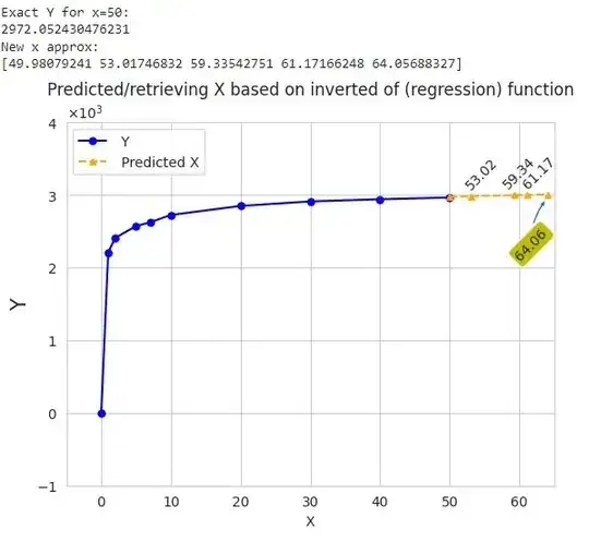
Basically, you just need to find the inversion of (regression function) formula that describes your model to find new Xs according to new given Ys. You don't need to fit a curve over your data necessarily.
Short note: I noticed that the data you have shown in pic for X-axis and Y-axis are not perfectly aligned when I put them in function:
# define the function
a = -0.007823866
b = 0.2984279
c = 0.1652267
d = 3512.422

def function(x, a, b, c, d):
    return d + (a - d)/(1 + (x/c)**b)

import math
print(f'f(0)= {math.ceil(function(0,a,b,c,d))}') #f(0)= 0
print(f'f(1)= {function(1,a,b,c,d):.1f}' )       #f(1)= 2217.0
print(f'f(2)= {function(2,a,b,c,d):.1f}' )       #f(2)= 2381.1
print(f'f(5)= {function(5,a,b,c,d):.1f}' )       #f(5)= 2579.9
print(f'f(7)= {function(7,a,b,c,d):.1f}' )       #f(7)= 2647.0
print(f'f(10)={function(10,a,b,c,d):.1f}' )      #f(10)=2714.6
print(f'f(20)={function(20,a,b,c,d):.1f}' )      #f(20)=2834.9
print(f'f(30)={function(30,a,b,c,d):.1f}' )      #f(30)=2898.6
print(f'f(40)={function(40,a,b,c,d):.1f}' )      #f(40)=2940.9
print(f'f(50)={function(50,a,b,c,d):.1f}' )      #f(50)=2972.1
- Fitting curve using scipy package:
# fit a second degree polynomial to the data
import numpy as np
from scipy.optimize import curve_fit

# define the function
a = -0.007823866
b = 0.2984279
c = 0.1652267
d = 3512.422

def function(x, a, b, c, d):
    return d + (a - d)/(1 + (x/c)**b)


# choose the input and output variables
x_data, y_data = np.array(df.X), np.array(df.Y)
print(x_data)
print(y_data)


p0 = [a, b, c, d]

# perform the curve fit
popt, pcov = curve_fit(function, x_data, y_data , p0=p0)
#popt, _ = curve_fit(forward, x, y)

# summarize the parameter values
print(popt)

## plot the results
import matplotlib.pyplot as plt
import seaborn as sns
sns.set_style("whitegrid")

#plt.figure()
plt.plot(x_data, y_data, marker="o", ms=8 , label="Data"                  , c='b')
plt.plot(x_new, y_new,   marker="o", ms=8 , label='New Ys', linestyle='--', c='darkblue')
plt.plot(x_data, function(x_data, *popt),  linestyle=':', c='orange', marker="s", ms=5, label="Fitted Curve")
#just for show case once if we could extend our fit cure over new data
plt.plot(inverse(y_new),  y_new,  linestyle=':', c='orange', marker="^", ms=5, label="Fitted Curve over new Ys")

plt.ticklabel_format(axis="y", style="sci", scilimits=(0,0))
plt.xlim(-5, 65)
plt.ylim(-1000, 4000)
plt.ylabel('Y', fontsize=15)

plt.annotate(f'{x_new[1]:.2f}', xy=(2, 1), xytext=(x_new[1] -1 , y_new[1] +100), rotation=45)
plt.annotate(f'{x_new[2]:.2f}', xy=(2, 1), xytext=(x_new[2] -2 , y_new[2] +100), rotation=45)
plt.annotate(f'{x_new[3]:.2f}', xy=(2, 1), xytext=(x_new[3] -1 , y_new[3] +100), rotation=45)
plt.annotate(f'{x_new[4]:.2f}', xy=(x_new[4], y_new[4]-50), xytext=(x_new[4] -5 , y_new[4] -900), rotation=45, bbox=dict(boxstyle="round", fc="y"), arrowprops=dict(arrowstyle="simple", connectionstyle="arc3,rad=-0.2"))


plt.title('Curve-Fitting with SciPy-optimize')
plt.legend(loc = "best")
plt.show()
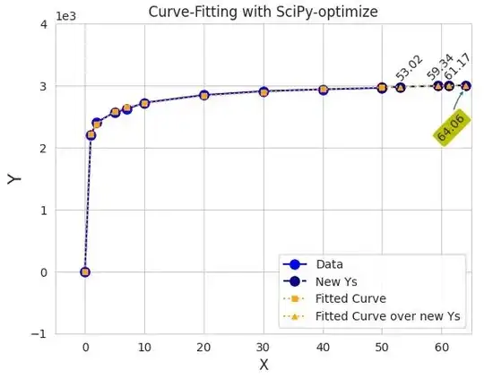
here my observation shows that when you set p0 within curve_fit() it perfectly fit over data.
According to DRY
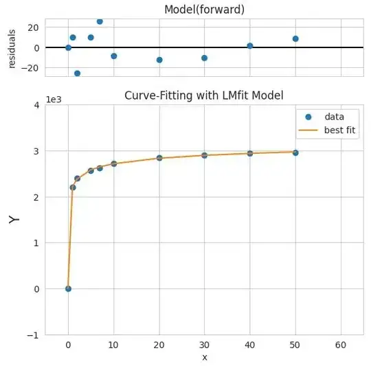
- Fitting curve using lmfit package check its docs:
#!pip install lmfit
import numpy as np
from lmfit import Model

a = -0.007823866
b = 0.2984279
c = 0.1652267
d = 3512.422

def forward(x):
    return d + (a - d)/(1 + (x/c)**b)

# create model from your model function
mymodel = Model(forward)

# create initial set of named parameters from argument of your function
params = mymodel.make_params(a=a, b=b, c=c, d=d)

# choose the input and output variables
x_data, y_data = df.X, df.Y

# run fit, get result
result = mymodel.fit(y_data, params, x=x_data)

# print out full fit report: fit statistics, best-fit values, uncertainties
#print(result.fit_report())  #error: ValueError: max() arg is an empty sequence

# make a stacked plot of residual and data + fit
import matplotlib.pyplot as plt
import seaborn as sns
sns.set_style("whitegrid")

plt.figure()
result.plot()
plt.xlim(-5, 65)
plt.ylim(-1000, 4000)
plt.ylabel('Y', fontsize=15)
plt.ticklabel_format(axis="y", style="sci", scilimits=(0,0))

plt.title('Curve-Fitting with LMfit Model')
plt.legend(loc = "best")
plt.show()