I have a dataframe with water levels. However, each water level is represented in mAOD (i.e. meters above sea level). Because of the positioning of each dip well this means the scale of the data is quite spread out. Is there an easy way to standardise the scale so they are all comparable. i.e. each curves starts at 0 and then fluctates from that point.
What my data currently looks like
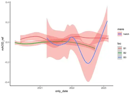
each line represents one of the dipwells.

library(ggplot2)
dataPlot <- dfDay %>%
  ggplot(aes(x=only_date, y=mAOD, colour=loc, fill=mere)) +
  geom_smooth() +
  theme_classic()

plot(dataPlot)
UPDATED Example Data
        structure(list(loc = c("B1", "B1", "B1", "B1", "B1", "B1", "B1",
"B1", "B1", "B1", "B2", "B2", "B2", "B2", "B2", "B2", "B2", "B2",
"B2", "B2", "B3", "B3", "B3", "B3", "B3", "B3", "B3", "B3", "B3",
"B3"), only_date = structure(c(18892, 18569, 19364, 19413, 18401,
18993, 19105, 19024, 18884, 18866, 18658, 19001, 19179, 18343,
18338, 18487, 18689, 18608, 18410, 19259, 18885, 18997, 19378,
19399, 18856, 18704, 18950, 18985, 19312, 19195), class = "Date"),
    mAOD = c(76.4009708333333, 76.4595041666667, 76.4425658333333,
    76.434795, 76.4279583333333, 76.4543291666667, 76.4517416666667,
    76.4566666666667, 76.4300916666667, 76.41275, 75.7512166666667,
    75.7413333333333, 75.7299333333333, 75.745425, 75.7511041666667,
    75.739375, 75.7554875, 75.7423666666667, 75.7269583333333,
    75.6779708333333, 74.5823541666667, 74.6553875, 74.7552704166667,
    74.74291375, 74.5447083333333, 74.6244708333333, 74.5701541666667,
    74.6534125, 74.7196166666667, 74.3292041666667), groundLevel = c(76.47,
    76.47, 76.47, 76.47, 76.47, 76.47, 76.47, 76.47, 76.47, 76.47,
    75.749, 75.749, 75.749, 75.749, 75.749, 75.749, 75.749, 75.749,
    75.749, 75.749, 74.729, 74.729, 74.729, 74.729, 74.729, 74.729,
    74.729, 74.729, 74.729, 74.729), rel_ground = c(-0.0690291666666673,
    -0.0104958333333342, -0.0274341666666687, -0.0352050000000019,
    -0.0420416666666655, -0.0156708333333331, -0.0182583333333331,
    -0.0133333333333325, -0.0399083333333348, -0.057250000000001,
    0.00221666666667394, -0.00766666666666005, -0.0190666666666578,
    -0.00357499999999256, 0.00210416666667553, -0.00962499999999267,
    0.00648750000000871, -0.00663333333332498, -0.0220416666666588,
    -0.0710291666666591, -0.146645833333328, -0.0736124999999953,
    0.0262704166666706, 0.0139137500000034, -0.184291666666664,
    -0.104529166666662, -0.158845833333329, -0.0755874999999957,
    -0.00938333333332804, -0.399795833333329), siteTemp = c(13.23875,
    10.5433333333333, 8.22045833333333, 7.974125, 9.68541666666667,
    8.85833333333333, 9.6625, 7.25166666666667, 13.60125, 13.40375,
    6.76, 7.89708333333333, 10.9870833333333, 8.06541666666667,
    8.22541666666667, 11.7675, 7.32291666666667, 8.53583333333333,
    10.0054166666667, 12.0283333333333, 13.3191666666667, 7.84541666666667,
    4.90841666666667, 4.7765, 13.20375, 5.71083333333333, 9.74416666666667,
    6.91041666666667, 10.2575, 12.5633333333333), baroTemp = c(14.2945833333333,
    6.2275, 9.48570833333333, 3.64475, 16.2891666666667, 12.4508333333333,
    11.3541666666667, 9.705, 15.1158333333333, 13.82625, 0.857083333333333,
    3.945, 16.6854166666667, 5.85416666666667, 11.6070833333333,
    22.1295833333333, 3.53916666666667, 6.82, 18.8345833333333,
    11.9033333333333, 14.9720833333333, 3.43416666666667, -1.21591666666667,
    8.36458333333333, 14.7433333333333, 7.04583333333333, 11.6491666666667,
    5.64458333333333, 6.84958333333333, 15.7204166666667), spi = c(0.30077434,
    -0.23930748, NaN, NaN, -2.6496189, -0.5860415, 0.33465025,
    1.0451335, 0.30077434, -0.43167603, 1.8315325, -0.5860415,
    -0.9746731, 1.3363327, 1.3363327, 1.6203027, 1.5484929, 0.9624635,
    -2.6496189, -0.70793974, 0.30077434, -0.5860415, NaN, NaN,
    -0.43167603, 1.5484929, -0.3823883, 0.35713777, 1.0100443,
    -0.9746731), beaverEvent = structure(c(2L, 2L, 3L, 3L, 1L,
    3L, 3L, 3L, 2L, 2L, 2L, 3L, 3L, 1L, 1L, 1L, 2L, 2L, 1L, 3L,
    2L, 3L, 3L, 3L, 2L, 2L, 3L, 3L, 3L, 3L), levels = c("BB",
    "AB", "D"), class = "factor"), mere = structure(c(2L, 2L,
    2L, 2L, 2L, 2L, 2L, 2L, 2L, 2L, 2L, 2L, 2L, 2L, 2L, 2L, 2L,
    2L, 2L, 2L, 2L, 2L, 2L, 2L, 2L, 2L, 2L, 2L, 2L, 2L), levels = c("chapel",
    "hatch", "coleCrose", "crose"), class = "factor"), damEvent = structure(c(1L,
    1L, 2L, 2L, 1L, 2L, 2L, 2L, 1L, 1L, 1L, 2L, 2L, 1L, 1L, 1L,
    1L, 1L, 1L, 2L, 1L, 2L, 2L, 2L, 1L, 1L, 2L, 2L, 2L, 2L), levels = c("1",
    "2"), class = "factor"), year = structure(c(2L, 1L, 3L, 3L,
    1L, 2L, 3L, 2L, 2L, 2L, 1L, 2L, 3L, 1L, 1L, 1L, 1L, 1L, 1L,
    3L, 2L, 2L, 3L, 3L, 2L, 2L, 2L, 2L, 3L, 3L), levels = c("1",
    "2", "3"), class = "factor"), ind = structure(c(1L, 1L, 1L,
    1L, 1L, 1L, 1L, 1L, 1L, 1L, 1L, 1L, 1L, 1L, 1L, 1L, 1L, 1L,
    1L, 1L, 1L, 1L, 1L, 1L, 1L, 1L, 1L, 1L, 1L, 1L), levels = c("ground",
    "surface"), class = "factor"), mAODscale = c(0.205100240746303,
    0.223349733604873, 0.218068708664052, 0.21564592220468, 0.213514389752922,
    0.221736274740243, 0.220929545307926, 0.22246505929987, 0.214179519333188,
    0.208772743331098, 0.00252021755022926, -0.000561203083351044,
    -0.00411548927790027, 0.000714494666301607, 0.00248514235751982,
    -0.00117177125273694, 0.00385177579197538, -0.000239030942907465,
    -0.00504303326287931, -0.0203163310660017, -0.361907137456628,
    -0.339136841982182, -0.307995397089215, -0.31184795232992,
    -0.37364433620216, -0.348776024571206, -0.365710847243781,
    -0.339752606476414, -0.319111505107548, -0.440834115540011
    ), sample = structure(c(2L, 2L, NA, NA, 2L, 2L, NA, 2L, 2L,
    2L, 2L, 2L, NA, 2L, 2L, 2L, 2L, 2L, 2L, NA, 2L, 2L, NA, NA,
    2L, 2L, 2L, 2L, NA, NA), levels = c("1", "2"), class = "factor")), class = c("grouped_df",
"tbl_df", "tbl", "data.frame"), row.names = c(NA, -30L), groups = structure(list(
    loc = c("B1", "B2", "B3"), .rows = structure(list(1:10, 11:20,
        21:30), ptype = integer(0), class = c("vctrs_list_of",
    "vctrs_vctr", "list"))), class = c("tbl_df", "tbl", "data.frame"
), row.names = c(NA, -3L), .drop = TRUE))