I have code to generate plots of interaction effects such as the following: (modelled in MTcars)
library(ggplot2)
library(tidyverse)

outcome_var_list = mtcars %>% select(qsec,hp) %>% names()
var_list = mtcars %>% select(cyl,wt) %>% names()


iterate <- sapply(outcome_var_list,function(k){

outcome_var_list = outcome_var_list[outcome_var_list == k]

test= mtcars %>%
  select(all_of(c(outcome_var_list, var_list)), drat)%>%
  pivot_longer(all_of(var_list))%>%
  reframe(broom::tidy(lm(as.matrix(pick(all_of(outcome_var_list)))~
               name/factor(drat):value + 0, data = .)))%>%
  select(term, estimate)%>%
  mutate(color = str_extract(term, "(?<=name)[^:]+"),
         xvar = as.numeric(str_extract(term, "[0-9.]+")))%>%
  drop_na()


test %>%  ggplot(aes(x=xvar, y=estimate, color = color)) + geom_line() + theme_light() + ggtitle(label = paste0("Model 1: ",k)) + theme(plot.title = element_text(hjust = 0.5))

ggsave(file=paste0("file_",k,".png"), width = 19, height = 7, units = "cm",path= "descriptive_1/test")

})
This generates plots such as the following:

Which plots the estimate of the interaction effect between the variable of interest and every factor level of "drat". Each separate plot repeats this for different outcome variables as listed.
I now want to slightly modify this to (presumably) use the marginaleffects package. I want to perform a similar function as above (evaluating and plotting each interaction within group for every outcome variable), but I need this to be slightly different. I now aim to plot the slope of the interaction effect (by subtracting the marginal effects) for each interaction with drat. I believe this can be done using the plot_slopes function, and setting factor levels of "drat" as the "condition" argument and the interaction with the var_list variable. However, I am unsure how to iterate this function similar to the above function. I also do not know how to plot these slopes together on the same ggplot2 plot as above.
Additionally, instead of plotting a continuous line, I would like to plot full confidence intervals, (lower and upper bound with point estimate) either connected with a line and shaded areas, or disconnected.
Is it possible to iterate over the plotting of the slopes similar to my previous example? Is this the right case for the marginaleffects package, or is there a base R/alternative solution that is more ideally suited to it? I also assume that to properly calculate these slopes I must switch from the : in the interaction term to * plot both the uninteracted effects in order to find the true slope. Is that the case?
Update
I see that this is indeed possible with marginaleffects, at least for manually plotting the interactions. For example, I can do the following:
library(marginaleffects)
lm1 = lm(data = mtcars, formula = hp ~ cyl*factor(drat))
lm2 = lm(data = mtcars, formula = hp ~ wt*factor(drat))
p1_data = plot_slopes(lm1, variables = "cyl", condition = "drat", draw = FALSE) %>% select(-cyl)
p2_data = plot_slopes(lm2, variables = "wt", condition = "drat", draw = FALSE) %>% select(-wt)
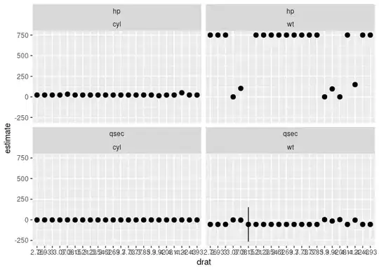
rbind(p1_data,p2_data) %>% ggplot() + geom_point(aes(x = factor(drat), y = predicted, color = term)) + geom_errorbar(aes(ymin = predicted_lo, ymax = predicted_hi, x = factor(drat), color = term))
Which generates the following plot:

Due to the scale, the error bars cannot be seen, but this is the correct plotting. However, my goal is to automate this, as in the above code, such that instead of individually plotting every regression for every variable in var_list, they are automatically fed in and generate lines with different colors for each variable. Then, I would iterate this over every single variable in outcome_var_list to produce multiple plots.