For exposure_1, I am trying to calculate and display the marginal effects of binary exposure_2 against the full model. I am unsure how to obtain these values. Once I have them, I need to translate them into tidy() format to display in my forest coefficient plot. I am also having difficulty creating this code.
Create dataframe and model
library(ggplot2)
library(dplyr)
library(marginaleffects)

# Set a random seed for reproducibility
set.seed(13)

# Number of rows in the dataframe
n <- 100

# Generate made-up data for exposures and outcome
exposure_1 <- sample(0:1, n, replace = TRUE)
exposure_2 <- sample(0:1, n, replace = TRUE)
exposure_3 <- sample(0:1, n, replace = TRUE)

# Generate made-up data for the primary outcome (assuming a binary outcome)
# The outcome could be generated based on some logic or model if needed
primary_outcome <- rbinom(n, 1, 0.3 + 0.2 * exposure_1 + 0.1 * exposure_2 - 0.1 * exposure_3)

# Generate made-up data for the community/grouping variable
enr_community <- sample(letters[1:5], n, replace = TRUE)

# Combine the generated data to create the dataframe
df <- data.frame(
  exposure_1 = exposure_1,
  exposure_2 = exposure_2,
  exposure_3 = exposure_3,
  primary_outcome = primary_outcome,
  enr_community = enr_community
)

logit_model_1 <- geeglm(formula = primary_outcome ~ exposure_1*exposure_2 + exposure_3 , family = binomial, id = enr_community, corstr = "independence", data = df)
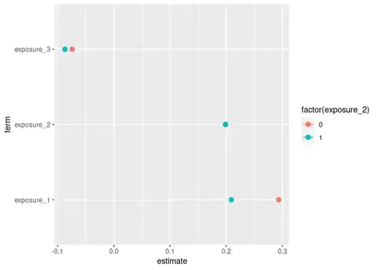
Create marginal effects (slopes) showing the estimates and 95% CIs for primary_outcome based on exposure_1 when exposure_2 is "0" and "1."
meffects <- slopes(logit_model_1,
   newdata = datagrid(primary_outcome = 1,
     exposure_2 = c(0, 1))) %>%
filter(term == "exposure_1")
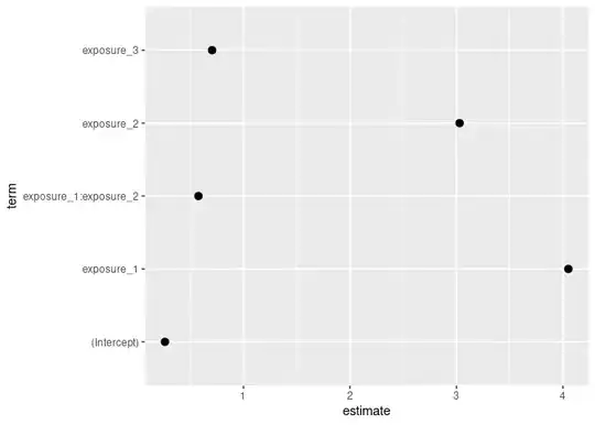
Transfer the logit model into a forest plot. Once meffects is transformed to show the estimates/CIs in relation to the full/base model, I will need to get it into tidy() format to add here.
lcf <- logit_model_1 %>%
  tidy(exponentiate = TRUE, conf.int = TRUE, conf.level = 0.95) %>%
  mutate(model = "Main Result") %>%
  mutate(exposure = "Exposure 1") %>%
  filter(term == "exposure_1")

lcftable <- lcf |>
  # round estimates and 95% CIs to 2 decimal places for journal specifications
  mutate(across(
    c(estimate, conf.low, conf.high, p.value),
    ~ str_pad(
      round(.x,2),
      width = 4,
      pad = "0",
      side = "right"
    ))) %>%
      mutate(estimate = case_when(
        estimate == "1000" ~ "1.00",
        TRUE ~ estimate
  )) %>%
  mutate(conf.low = case_when(
        conf.low == "1000" ~ "1.00",
        TRUE ~ conf.low
  )) %>%
  mutate(conf.high = case_when(
        conf.high == "2000" ~ "2.00",
        TRUE ~ conf.high
  )) %>%
  mutate(model = fct_rev(fct_relevel(model, "Model")))

lcftable <- lcftable %>%
  #convert back to characters
  mutate(estimate = format(estimate, n.small = 3),
    conf.low = format(conf.low, n.small = 3),
    conf.high = format(conf.high, n.small = 3),
    estimate_lab = paste0(estimate, " (", as.character(conf.low), " -", conf.high, ")")) |>
     mutate(p.value = as.numeric(p.value)) %>%
  # round p-values to two decimal places, except in cases where p < .001
  mutate(p.value = case_when(
    p.value < .001 ~ "<0.001",
    round(p.value, 2) == .05 ~ as.character(round(p.value,3)),
    p.value < .01 ~ str_pad( # if less than .01, go one more decimal place
      as.character(round(p.value, 3)),
      width = 4,
      pad = "0",
      side = "right"
    ),
    p.value > 0.995 ~ "1.00",
    TRUE ~ str_pad( # otherwise just round to 2 decimal places and pad string so that .2 reads as 0.20
      as.character(round(p.value, 2)),
      width = 4,
      pad = "0",
      side = "right"
    ))) %>%
   mutate(estimate = as.numeric(estimate),
    conf.low = as.numeric(conf.low),
    conf.high = as.numeric(conf.high))

lcfplot1 <- lcftable %>%
  ggplot(mapping = aes(x = estimate, xmin = conf.low, xmax = conf.high, y = model)) + #y = model rather than term
  geom_pointrange() +
 # scale_x_continuous(breaks = c(0, 1.0, 1.5, 2.0)) + #trans = scales::pseudo_log_trans(base = 10)
  geom_vline(xintercept = 1) +
  geom_point(size = 1.0) +
#adjust facet grid
  facet_wrap(exposure~., ncol = 1, scale = "free_y") +
  xlab("Incident Odds Ratio, IOR (95% Confidence Interval)") +
  ggtitle("Associations between exposures and outcome") +
  geom_text(aes(x = 3.5, label = estimate_lab), hjust = -0.5, size = 3) +
  geom_text(aes(x = 2.5, label = p.value), hjust = -3.5, size = 3) +
  coord_cartesian(xlim = c(-0.1, 7.0)) +
  scale_x_continuous(trans = "pseudo_log", breaks = c(-1.0, 0, 1.0, 2.0, 5.0)) +
  theme(panel.background = element_blank(),
        panel.spacing = unit(1, "lines"),
        panel.border = element_rect(fill = NA, color = "white"),
        strip.background = element_rect(colour="white", fill="white"),
        strip.placement = "outside",
        text = element_text(size = 12),
        strip.text = element_text(face = "bold.italic", size = 11, hjust = 0.33), #element_blank(),
        plot.title = element_text(face = "bold", size = 13, hjust = -11, vjust = 4),
        axis.title.x = element_text(size = 10, vjust = -1, hjust = 0.05),
        axis.title.y = element_blank(),
        panel.grid.major.x = element_line(color = "#D3D3D3",
                                  size = 0.3, linetype = 2),
        plot.margin = unit(c(1, 3, 0.5, 0.5), "inches")) +
  geom_errorbarh(height = 0)