0

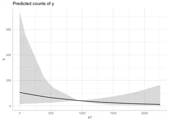
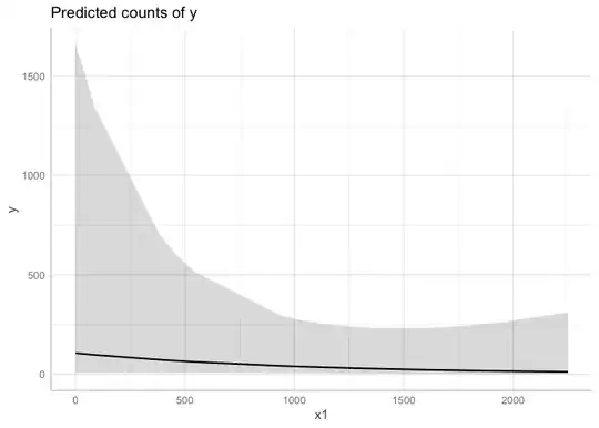
Is there any way to make a conditional plot using visreg fucntion when I have scaled my regressors? I want to plot my rescaled response along with 95%CIs, prediction curve, and partial residuals.

install.packages("lme4")
library("lme4")    
y <- c(18, 0, 2, 0,  0,  0,  2,  0,  0,  1,  7,  0,  0,  0,  0,  0,  0,  0,  0)
x1 <- c(501, 1597, 1156, 1134, 1924,  507, 1022,  0,  92, 1729, 85, 963, 544, 1315, 2250, 1366,  458,  385,  930)
x2 <- c(0,  92,  959, 1146,  900,  0,  276, 210,  980, 8, 0, 473, 0, 255, 1194, 542, 983, 331,  923)
x3 <- c("site1", "site1", "site2","site2","site3","site3","site4","site4","site5","site5","site6","site7","site8","site9","site10","site11","site12","site13","site14")

offset_1 <- c(59, 34, 33, 35, 60, 58, 59, 33, 34, 61, 58, 58, 55, 26, 26, 18, 26, 26, 26)
data_1 <- data.frame(y,x1,x2,offset_1)

m1 <- glmer.nb(y ~ -1 + scale(x1) + scale(x2) + + (1|x3) + offset(log(offset_1)), data=data_1)
summary(m1)
visreg(m1, "x1", scale="response", cond=list(offset_1=1), partial=TRUE,
       rug=2,line=list(lwd=0.5, col="black"), points=list(cex=1.4, lwd=0.1, col="black", pch=21))
  • From the `visreg` [mixed models vignette](http://pbreheny.github.io/visreg/articles/web/mixed.html): "visreg can be used with mixed models, for example from the nlme or lme4 packages, although it is worth noting that these packages are unable to incorporate uncertainty about random effects into predictions, and therefore do not offer confidence intervals, meaning that visreg plots will lack confidence bands. " – DaveArmstrong Aug 12 '23 at 01:36

1 Answers1

1

As I mentioned in the comment above, visreg will not do what you want. You could use the ggeffects package to do it.

library("lme4")    
#> Loading required package: Matrix
y <- c(18, 0, 2, 0,  0,  0,  2,  0,  0,  1,  7,  0,  0,  0,  0,  0,  0,  0,  0)
x1 <- c(501, 1597, 1156, 1134, 1924,  507, 1022,  0,  92, 1729, 85, 963, 544, 1315, 2250, 1366,  458,  385,  930)
x2 <- c(0,  92,  959, 1146,  900,  0,  276, 210,  980, 8, 0, 473, 0, 255, 1194, 542, 983, 331,  923)
x3 <- c("site1", "site1", "site2","site2","site3","site3","site4","site4","site5","site5","site6","site7","site8","site9","site10","site11","site12","site13","site14")

offset_1 <- c(59, 34, 33, 35, 60, 58, 59, 33, 34, 61, 58, 58, 55, 26, 26, 18, 26, 26, 26)
data_1 <- data.frame(y,x1,x2,offset_1)

m1 <- glmer.nb(y ~ -1 + scale(x1) + scale(x2) + + (1|x3) + offset(log(offset_1)), data=data_1)
#> Warning in theta.ml(Y, mu, weights = object@resp$weights, limit = limit, :
#> iteration limit reached
summary(m1)
#> Generalized linear mixed model fit by maximum likelihood (Laplace
#>   Approximation) [glmerMod]
#>  Family: Negative Binomial(260.1065)  ( log )
#> Formula: y ~ -1 + scale(x1) + scale(x2) + +(1 | x3) + offset(log(offset_1))
#>    Data: data_1
#> 
#>      AIC      BIC   logLik deviance df.resid 
#>     86.0     89.8    -39.0     78.0       15 
#> 
#> Scaled residuals: 
#>     Min      1Q  Median      3Q     Max 
#> -1.2281 -0.2982 -0.1695 -0.0254  1.9513 
#> 
#> Random effects:
#>  Groups Name        Variance Std.Dev.
#>  x3     (Intercept) 104.6    10.23   
#> Number of obs: 19, groups:  x3, 14
#> 
#> Fixed effects:
#>           Estimate Std. Error z value Pr(>|z|)
#> scale(x1)  -0.6437     0.6776  -0.950    0.342
#> scale(x2)  -3.8961     4.1772  -0.933    0.351
#> 
#> Correlation of Fixed Effects:
#>           scl(1)
#> scale(x2) -0.740

library(ggeffects)
## confidence interval for slope, assuming
## 0 random effect variance. 
g1 <- ggpredict(m1, "x1 [all]", type="fixed")
plot(g1)


## prediction intervals including 
## random effect variance
g2 <- ggpredict(m1, "x1 [all]", type="random")
plot(g2)

Created on 2023-08-12 with reprex v2.0.2

DaveArmstrong
  • 18,377
  • 2
  • 13
  • 25