Principal component analysis in Python

Question

I'd like to use principal component analysis (PCA) for dimensionality reduction. Does numpy or scipy already have it, or do I have to roll my own using numpy.linalg.eigh?

I don't just want to use singular value decomposition (SVD) because my input data are quite high-dimensional (~460 dimensions), so I think SVD will be slower than computing the eigenvectors of the covariance matrix.

I was hoping to find a premade, debugged implementation that already makes the right decisions for when to use which method, and which maybe does other optimizations that I don't know about.

Answer 1

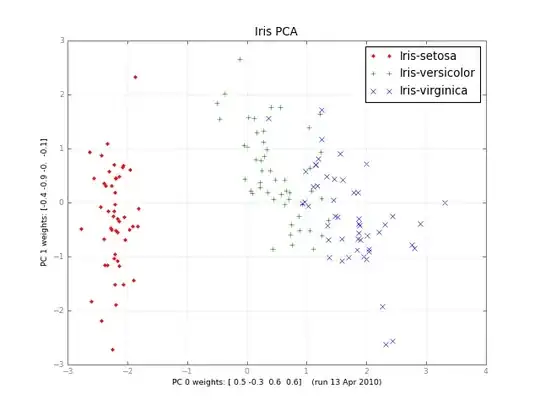
Months later, here's a small class PCA, and a picture:

#!/usr/bin/env python
""" a small class for Principal Component Analysis
Usage:
    p = PCA( A, fraction=0.90 )
In:
    A: an array of e.g. 1000 observations x 20 variables, 1000 rows x 20 columns
    fraction: use principal components that account for e.g.
        90 % of the total variance

Out:
    p.U, p.d, p.Vt: from numpy.linalg.svd, A = U . d . Vt
    p.dinv: 1/d or 0, see NR
    p.eigen: the eigenvalues of A*A, in decreasing order (p.d**2).
        eigen[j] / eigen.sum() is variable j's fraction of the total variance;
        look at the first few eigen[] to see how many PCs get to 90 %, 95 % ...
    p.npc: number of principal components,
        e.g. 2 if the top 2 eigenvalues are >= `fraction` of the total.
        It's ok to change this; methods use the current value.

Methods:
    The methods of class PCA transform vectors or arrays of e.g.
    20 variables, 2 principal components and 1000 observations,
    using partial matrices U' d' Vt', parts of the full U d Vt:
    A ~ U' . d' . Vt' where e.g.
        U' is 1000 x 2
        d' is diag([ d0, d1 ]), the 2 largest singular values
        Vt' is 2 x 20.  Dropping the primes,

    d . Vt      2 principal vars = p.vars_pc( 20 vars )
    U           1000 obs = p.pc_obs( 2 principal vars )
    U . d . Vt  1000 obs, p.obs( 20 vars ) = pc_obs( vars_pc( vars ))
        fast approximate A . vars, using the `npc` principal components

    Ut              2 pcs = p.obs_pc( 1000 obs )
    V . dinv        20 vars = p.pc_vars( 2 principal vars )
    V . dinv . Ut   20 vars, p.vars( 1000 obs ) = pc_vars( obs_pc( obs )),
        fast approximate Ainverse . obs: vars that give ~ those obs.


Notes:
    PCA does not center or scale A; you usually want to first
        A -= A.mean(A, axis=0)
        A /= A.std(A, axis=0)
    with the little class Center or the like, below.

See also:
    http://en.wikipedia.org/wiki/Principal_component_analysis
    http://en.wikipedia.org/wiki/Singular_value_decomposition
    Press et al., Numerical Recipes (2 or 3 ed), SVD
    PCA micro-tutorial
    iris-pca .py .png

"""

from __future__ import division
import numpy as np
dot = np.dot
    # import bz.numpyutil as nu
    # dot = nu.pdot

__version__ = "2010-04-14 apr"
__author_email__ = "denis-bz-py at t-online dot de"

#...............................................................................
class PCA:
    def __init__( self, A, fraction=0.90 ):
        assert 0 <= fraction <= 1
            # A = U . diag(d) . Vt, O( m n^2 ), lapack_lite --
        self.U, self.d, self.Vt = np.linalg.svd( A, full_matrices=False )
        assert np.all( self.d[:-1] >= self.d[1:] )  # sorted
        self.eigen = self.d**2
        self.sumvariance = np.cumsum(self.eigen)
        self.sumvariance /= self.sumvariance[-1]
        self.npc = np.searchsorted( self.sumvariance, fraction ) + 1
        self.dinv = np.array([ 1/d if d > self.d[0] * 1e-6  else 0
                                for d in self.d ])

    def pc( self ):
        """ e.g. 1000 x 2 U[:, :npc] * d[:npc], to plot etc. """
        n = self.npc
        return self.U[:, :n] * self.d[:n]

    # These 1-line methods may not be worth the bother;
    # then use U d Vt directly --

    def vars_pc( self, x ):
        n = self.npc
        return self.d[:n] * dot( self.Vt[:n], x.T ).T  # 20 vars -> 2 principal

    def pc_vars( self, p ):
        n = self.npc
        return dot( self.Vt[:n].T, (self.dinv[:n] * p).T ) .T  # 2 PC -> 20 vars

    def pc_obs( self, p ):
        n = self.npc
        return dot( self.U[:, :n], p.T )  # 2 principal -> 1000 obs

    def obs_pc( self, obs ):
        n = self.npc
        return dot( self.U[:, :n].T, obs ) .T  # 1000 obs -> 2 principal

    def obs( self, x ):
        return self.pc_obs( self.vars_pc(x) )  # 20 vars -> 2 principal -> 1000 obs

    def vars( self, obs ):
        return self.pc_vars( self.obs_pc(obs) )  # 1000 obs -> 2 principal -> 20 vars


class Center:
    """ A -= A.mean() /= A.std(), inplace -- use A.copy() if need be
        uncenter(x) == original A . x
    """
        # mttiw
    def __init__( self, A, axis=0, scale=True, verbose=1 ):
        self.mean = A.mean(axis=axis)
        if verbose:
            print "Center -= A.mean:", self.mean
        A -= self.mean
        if scale:
            std = A.std(axis=axis)
            self.std = np.where( std, std, 1. )
            if verbose:
                print "Center /= A.std:", self.std
            A /= self.std
        else:
            self.std = np.ones( A.shape[-1] )
        self.A = A

    def uncenter( self, x ):
        return np.dot( self.A, x * self.std ) + np.dot( x, self.mean )


#...............................................................................
if __name__ == "__main__":
    import sys

    csv = "iris4.csv"  # wikipedia Iris_flower_data_set
        # 5.1,3.5,1.4,0.2  # ,Iris-setosa ...
    N = 1000
    K = 20
    fraction = .90
    seed = 1
    exec "\n".join( sys.argv[1:] )  # N= ...
    np.random.seed(seed)
    np.set_printoptions( 1, threshold=100, suppress=True )  # .1f
    try:
        A = np.genfromtxt( csv, delimiter="," )
        N, K = A.shape
    except IOError:
        A = np.random.normal( size=(N, K) )  # gen correlated ?

    print "csv: %s  N: %d  K: %d  fraction: %.2g" % (csv, N, K, fraction)
    Center(A)
    print "A:", A

    print "PCA ..." ,
    p = PCA( A, fraction=fraction )
    print "npc:", p.npc
    print "% variance:", p.sumvariance * 100

    print "Vt[0], weights that give PC 0:", p.Vt[0]
    print "A . Vt[0]:", dot( A, p.Vt[0] )
    print "pc:", p.pc()

    print "\nobs <-> pc <-> x: with fraction=1, diffs should be ~ 0"
    x = np.ones(K)
    # x = np.ones(( 3, K ))
    print "x:", x
    pc = p.vars_pc(x)  # d' Vt' x
    print "vars_pc(x):", pc
    print "back to ~ x:", p.pc_vars(pc)

    Ax = dot( A, x.T )
    pcx = p.obs(x)  # U' d' Vt' x
    print "Ax:", Ax
    print "A'x:", pcx
    print "max |Ax - A'x|: %.2g" % np.linalg.norm( Ax - pcx, np.inf )

    b = Ax  # ~ back to original x, Ainv A x
    back = p.vars(b)
    print "~ back again:", back
    print "max |back - x|: %.2g" % np.linalg.norm( back - x, np.inf )

# end pca.py

Answer 2

PCA using numpy.linalg.svd is super easy. Here's a simple demo:

import numpy as np
import matplotlib.pyplot as plt
from scipy.misc import lena

# the underlying signal is a sinusoidally modulated image
img = lena()
t = np.arange(100)
time = np.sin(0.1*t)
real = time[:,np.newaxis,np.newaxis] * img[np.newaxis,...]

# we add some noise
noisy = real + np.random.randn(*real.shape)*255

# (observations, features) matrix
M = noisy.reshape(noisy.shape[0],-1)

# singular value decomposition factorises your data matrix such that:
# 
#   M = U*S*V.T     (where '*' is matrix multiplication)
# 
# * U and V are the singular matrices, containing orthogonal vectors of
#   unit length in their rows and columns respectively.
#
# * S is a diagonal matrix containing the singular values of M - these 
#   values squared divided by the number of observations will give the 
#   variance explained by each PC.
#
# * if M is considered to be an (observations, features) matrix, the PCs
#   themselves would correspond to the rows of S^(1/2)*V.T. if M is 
#   (features, observations) then the PCs would be the columns of
#   U*S^(1/2).
#
# * since U and V both contain orthonormal vectors, U*V.T is equivalent 
#   to a whitened version of M.

U, s, Vt = np.linalg.svd(M, full_matrices=False)
V = Vt.T

# PCs are already sorted by descending order 
# of the singular values (i.e. by the
# proportion of total variance they explain)

# if we use all of the PCs we can reconstruct the noisy signal perfectly
S = np.diag(s)
Mhat = np.dot(U, np.dot(S, V.T))
print "Using all PCs, MSE = %.6G" %(np.mean((M - Mhat)**2))

# if we use only the first 20 PCs the reconstruction is less accurate
Mhat2 = np.dot(U[:, :20], np.dot(S[:20, :20], V[:,:20].T))
print "Using first 20 PCs, MSE = %.6G" %(np.mean((M - Mhat2)**2))

fig, [ax1, ax2, ax3] = plt.subplots(1, 3)
ax1.imshow(img)
ax1.set_title('true image')
ax2.imshow(noisy.mean(0))
ax2.set_title('mean of noisy images')
ax3.imshow((s[0]**(1./2) * V[:,0]).reshape(img.shape))
ax3.set_title('first spatial PC')
plt.show()

Answer 3

You can use sklearn:

import sklearn.decomposition as deco
import numpy as np

x = (x - np.mean(x, 0)) / np.std(x, 0) # You need to normalize your data first
pca = deco.PCA(n_components) # n_components is the components number after reduction
x_r = pca.fit(x).transform(x)
print ('explained variance (first %d components): %.2f'%(n_components, sum(pca.explained_variance_ratio_)))

Answer 4

matplotlib.mlab has a PCA implementation.

Answer 5

You might have a look at MDP.

I have not had the chance to test it myself, but I've bookmarked it exactly for the PCA functionality.

Answer 6

SVD should work fine with 460 dimensions. It takes about 7 seconds on my Atom netbook. The eig() method takes more time (as it should, it uses more floating point operations) and will almost always be less accurate.

If you have less than 460 examples then what you want to do is diagonalize the scatter matrix (x - datamean)^T(x - mean), assuming your data points are columns, and then left-multiplying by (x - datamean). That might be faster in the case where you have more dimensions than data.

Answer 7

You can quite easily "roll" your own using scipy.linalg (assuming a pre-centered dataset data):

covmat = data.dot(data.T)
evs, evmat = scipy.linalg.eig(covmat)

Then evs are your eigenvalues, and evmat is your projection matrix.

If you want to keep d dimensions, use the first d eigenvalues and first d eigenvectors.

Given that scipy.linalg has the decomposition and numpy the matrix multiplications, what else do you need?

Answer 8

I just finish reading the book Machine Learning: An Algorithmic Perspective. All code examples in the book was written by Python(and almost with Numpy). The code snippet of chatper10.2 Principal Components Analysis maybe worth a reading. It use numpy.linalg.eig.
By the way, I think SVD can handle 460 * 460 dimensions very well. I have calculate a 6500*6500 SVD with numpy/scipy.linalg.svd on a very old PC:Pentium III 733mHz. To be honest, the script needs a lot of memory(about 1.xG) and a lot of time(about 30 minutes) to get the SVD result. But I think 460*460 on a modern PC will not be a big problem unless u need do SVD a huge number of times.

Answer 9

You do not need full Singular Value Decomposition (SVD) at it computes all eigenvalues and eigenvectors and can be prohibitive for large matrices. scipy and its sparse module provide generic linear algrebra functions working on both sparse and dense matrices, among which there is the eig* family of functions :

http://docs.scipy.org/doc/scipy/reference/sparse.linalg.html#matrix-factorizations

Scikit-learn provides a Python PCA implementation which only support dense matrices for now.

Timings :

In [1]: A = np.random.randn(1000, 1000)

In [2]: %timeit scipy.sparse.linalg.eigsh(A)
1 loops, best of 3: 802 ms per loop

In [3]: %timeit np.linalg.svd(A)
1 loops, best of 3: 5.91 s per loop

Answer 10

Here is another implementation of a PCA module for python using numpy, scipy and C-extensions. The module carries out PCA using either a SVD or the NIPALS (Nonlinear Iterative Partial Least Squares) algorithm which is implemented in C.

Answer 11

If you're working with 3D vectors, you can apply SVD concisely using the toolbelt vg. It's a light layer on top of numpy.

import numpy as np
import vg

vg.principal_components(data)

There's also a convenient alias if you only want the first principal component:

vg.major_axis(data)

I created the library at my last startup, where it was motivated by uses like this: simple ideas which are verbose or opaque in NumPy.