2

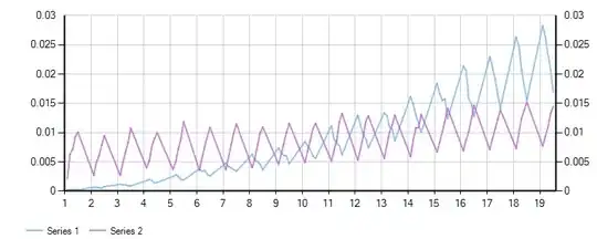
I'm trying to do something similar to what's outlined in this post: MATLAB, Filling in the area between two sets of data, lines in one figure but running into a roadblock. I'm trying to shade the area of a graph that represents the mean +/- standard deviation. The variable definitions are a bit complicated but it boils down to this code, and when plotted without shading, I get the screenshot below:

x = linspace(0, 100, 101)';    
mean = torqueRnormMean(:,1);
meanPlusSTD = torqueRnormMean(:,1) + torqueRnormStd(:,1);
meanMinusSTD = torqueRnormMean(:,1) - torqueRnormStd(:,1);
plot(x, mean, 'k', 'LineWidth', 2)
plot(x, meanPlusSTD, 'k--')
plot(x, meanMinusSTD, 'k--')

mean and std

But when I try to implement shading just on the lower half of the graph (between mean and meanMinusSTD) by adding the code below, I get a plot that looks like this:

fill( [x fliplr(x)],  [mean fliplr(meanMinusSTD)], 'y', 'LineStyle','--');

shaded

It's obviously not shading the correct area of the graph, and new near-horizontal lines are being created close to 0 that are messing with the shading.

Any thoughts? I'm stumped.

Community
  • 1
  • 1
dustynrobots
  • 311
  • 4
  • 8
  • 20

4 Answers4

7

You may be getting a problem with using mean as a variable, since it's also a reserved MATLAB command. Try clearing the variable space and then using a unique variable name.

As for the second problem, you want

fill( [x fliplr(x)],  [meanUniqueName fliplr(meanMinusSTD)], 'y', 'LineStyle','--');

You also don't need to do this in two steps, but can do it all at once. A code snippet from a script I'm currently working on does the exact same thing and contains the lines:

    avar = allan(DATA, tau);
    xFill = [avar.tau1 fliplr(avar.tau1)];
    yFill = [avar.sig2+avar.sig2err fliplr(avar.sig2-avar.sig2err)];

    figure(2);
    fill(xFill,yFill,'y','LineStyle','--')
    line(avar.tau1,avar.sig2);

So I fill the area between the two error lines, and then draw the data line on top.

craigim
  • 3,884
  • 1
  • 22
  • 42
  • The LineStyle addition worked (thanks!) but even after clearing the variable space and changing the word mean to meanVar I get the same results. – dustynrobots Nov 11 '13 at 16:50
  • Just looking at the graph, it looks like you're filling the area between `torqueRnormStd` and `torqueRnormMean-torqueRnormStd`. That's not what you have written here, but that's what your graph looks like. Perhaps you transposed variable names in your code somewhere? – craigim Nov 11 '13 at 17:17
  • I checked the code and am pretty sure not variable names got transposed. Also I know it's another step but I also have two plotting options: one that does this shading, and another that plots all the individual lines of the dataset, but in either case I show the mean, mean+SD, and mean-SD lines, so they're defined first. – dustynrobots Nov 11 '13 at 18:02
6

It turned out to be a column vs row vector issue. For some reason using the fill method above with flipud with the original column vectors doesn't work, but transposing the original variables then using fliplr does. Go figure. Here's the code in case it helps someone else:

x = linspace(0,100, 101);
mean = torqueRnormMean(:,DOF)';
meanPlusSTD = torqueRnormMean(:,DOF)' + torqueRnormStd(:,DOF)';
meanMinusSTD = torqueRnormMean(:,DOF)' - torqueRnormStd(:,DOF)';
fill( [x fliplr(x)],  [meanPlusSTD fliplr(meanMinusSTD)], 'k');
alpha(.25);
plot(x, mean, 'k', 'LineWidth', 2)
plot(x, meanPlusSTD, 'k')
plot(x, meanMinusSTD, 'k')

Note that I removed the dotted line and just used thin vs. thick lines to denote standard deviation and mean. I did this because the line style was inconsistent. This code is in a loop where DOF runs from 1:9, and in some of the subplots both std curves would be dashed and in some just the top or bottom. It didn't matter enough to me to have them dashed so I kept it simple. Now this is an example of the graph I get:

enter image description here

dustynrobots
  • 311
  • 4
  • 8
  • 20
  • Hi, I suggest you post your full solution and make your answer the accepted answer. This way, if people with the same question come across your post, they can easily find the correct answer. – A. Donda Nov 11 '13 at 21:17
  • Okay it says I need to wait 2 days to mark my own as the accepted answer, but I'll post the full code in the mean time. – dustynrobots Nov 11 '13 at 21:37
4

Another possibility:

x = 1:1000; % example x values
y_upper = 5+sin(2*pi/200*x); % example upper curve
y_lower = 2+sin(2*pi/230*x); % example lower curve
bar(x, y_upper, 1, 'b', 'edgecolor', 'b');
hold on
bar(x, y_lower, 1, 'w', 'edgecolor', 'w');
axis([0 1000 0 7])

It uses bar (with unit width and same-color edges) to fill the upper curve, and then a second bar to "remove" (plot in white) the lower part.

enter image description here

Luis Mendo
  • 110,752
  • 13
  • 76
  • 147
3

One thing that you appear to be doing wrong is that you're applying fliplr to column vectors. That will have no effect. The example you cited uses row vectors. You also concatenate them into a matrix instead of into a single vector like the example. I think that the equivalent with column vectors would be:

fill( [x;flipud(x)],  [mean;flipud(meanMinusSTD)], 'y');
horchler
  • 18,384
  • 4
  • 37
  • 73
  • I just tried that (thanks for the catch, it does make sense) but it doesn't have any affect on the graph unfortunately. – dustynrobots Nov 11 '13 at 16:49