image information along a polar coordinate system

Question

I have a set of png images that I would like to process with Python and associated tools. Each image represents a physical object with known dimensions.

In each image there is a specific feature of the object at a certain pixel/physical location. The location is different for each image.

I would like to impose a polar coordinate system on a given image with the origin at the location of this feature.

I would then like to be able to get the following information: - the image intensity as a function of radial position for a given polar angle - the image intensity as a function of radial position when values are averaged over all polar angles.

I am experienced in Python programming and the use of many functions in NumPy and SciPy, but I am a complete novice when it comes to image analysis.

I would appreciate any advice you can give me on possible approaches to use to solve this problem.

Thank you.

Answer 1

What you're describing isn't exactly image processing in the traditional sense, but it's fairly easy to do with numpy, etc.

Here's a rather large example doing some of the things you mentioned to get you pointed in the right direction... Note that the example images all show results for the origin at the center of the image, but the functions take an origin argument, so you should be able to directly adapt things for your purposes.

import numpy as np
import scipy as sp
import scipy.ndimage

import Image

import matplotlib.pyplot as plt

def main():
    im = Image.open('mri_demo.png')
    im = im.convert('RGB')
    data = np.array(im)

    plot_polar_image(data, origin=None)
    plot_directional_intensity(data, origin=None)

    plt.show()

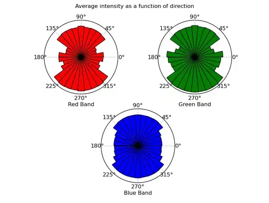
def plot_directional_intensity(data, origin=None):
    """Makes a cicular histogram showing average intensity binned by direction
    from "origin" for each band in "data" (a 3D numpy array). "origin" defaults
    to the center of the image."""
    def intensity_rose(theta, band, color):
        theta, band = theta.flatten(), band.flatten()
        intensities, theta_bins = bin_by(band, theta)
        mean_intensity = map(np.mean, intensities)
        width = np.diff(theta_bins)[0]
        plt.bar(theta_bins, mean_intensity, width=width, color=color)
        plt.xlabel(color + ' Band')
        plt.yticks([])

    # Make cartesian coordinates for the pixel indicies
    # (The origin defaults to the center of the image)
    x, y = index_coords(data, origin)

    # Convert the pixel indices into polar coords.
    r, theta = cart2polar(x, y)

    # Unpack bands of the image
    red, green, blue = data.T

    # Plot...
    plt.figure()

    plt.subplot(2,2,1, projection='polar')
    intensity_rose(theta, red, 'Red')

    plt.subplot(2,2,2, projection='polar')
    intensity_rose(theta, green, 'Green')

    plt.subplot(2,1,2, projection='polar')
    intensity_rose(theta, blue, 'Blue')

    plt.suptitle('Average intensity as a function of direction')

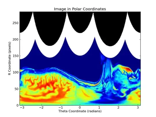
def plot_polar_image(data, origin=None):
    """Plots an image reprojected into polar coordinages with the origin
    at "origin" (a tuple of (x0, y0), defaults to the center of the image)"""
    polar_grid, r, theta = reproject_image_into_polar(data, origin)
    plt.figure()
    plt.imshow(polar_grid, extent=(theta.min(), theta.max(), r.max(), r.min()))
    plt.axis('auto')
    plt.ylim(plt.ylim()[::-1])
    plt.xlabel('Theta Coordinate (radians)')
    plt.ylabel('R Coordinate (pixels)')
    plt.title('Image in Polar Coordinates')

def index_coords(data, origin=None):
    """Creates x & y coords for the indicies in a numpy array "data".
    "origin" defaults to the center of the image. Specify origin=(0,0)
    to set the origin to the lower left corner of the image."""
    ny, nx = data.shape[:2]
    if origin is None:
        origin_x, origin_y = nx // 2, ny // 2
    else:
        origin_x, origin_y = origin
    x, y = np.meshgrid(np.arange(nx), np.arange(ny))
    x -= origin_x
    y -= origin_y
    return x, y

def cart2polar(x, y):
    r = np.sqrt(x**2 + y**2)
    theta = np.arctan2(y, x)
    return r, theta

def polar2cart(r, theta):
    x = r * np.cos(theta)
    y = r * np.sin(theta)
    return x, y


def bin_by(x, y, nbins=30):
    """Bin x by y, given paired observations of x & y.
    Returns the binned "x" values and the left edges of the bins."""
    bins = np.linspace(y.min(), y.max(), nbins+1)
    # To avoid extra bin for the max value
    bins[-1] += 1 

    indicies = np.digitize(y, bins)

    output = []
    for i in xrange(1, len(bins)):
        output.append(x[indicies==i])

    # Just return the left edges of the bins
    bins = bins[:-1]

    return output, bins

def reproject_image_into_polar(data, origin=None):
    """Reprojects a 3D numpy array ("data") into a polar coordinate system.
    "origin" is a tuple of (x0, y0) and defaults to the center of the image."""
    ny, nx = data.shape[:2]
    if origin is None:
        origin = (nx//2, ny//2)

    # Determine that the min and max r and theta coords will be...
    x, y = index_coords(data, origin=origin)
    r, theta = cart2polar(x, y)

    # Make a regular (in polar space) grid based on the min and max r & theta
    r_i = np.linspace(r.min(), r.max(), nx)
    theta_i = np.linspace(theta.min(), theta.max(), ny)
    theta_grid, r_grid = np.meshgrid(theta_i, r_i)

    # Project the r and theta grid back into pixel coordinates
    xi, yi = polar2cart(r_grid, theta_grid)
    xi += origin[0] # We need to shift the origin back to 
    yi += origin[1] # back to the lower-left corner...
    xi, yi = xi.flatten(), yi.flatten()
    coords = np.vstack((xi, yi)) # (map_coordinates requires a 2xn array)

    # Reproject each band individually and the restack
    # (uses less memory than reprojection the 3-dimensional array in one step)
    bands = []
    for band in data.T:
        zi = sp.ndimage.map_coordinates(band, coords, order=1)
        bands.append(zi.reshape((nx, ny)))
    output = np.dstack(bands)
    return output, r_i, theta_i

if __name__ == '__main__':
    main()

Original Image:

Projected into polar coordinates:

Intensity as a function of direction from the center of the image:

Answer 2

Here's my take using scipy's geometric_transform method:

topolar.py

import numpy as np
from scipy.ndimage.interpolation import geometric_transform

def topolar(img, order=1):
    """
    Transform img to its polar coordinate representation.

    order: int, default 1
        Specify the spline interpolation order. 
        High orders may be slow for large images.
    """
    # max_radius is the length of the diagonal 
    # from a corner to the mid-point of img.
    max_radius = 0.5*np.linalg.norm( img.shape )

    def transform(coords):
        # Put coord[1] in the interval, [-pi, pi]
        theta = 2*np.pi*coords[1] / (img.shape[1] - 1.)

        # Then map it to the interval [0, max_radius].
        #radius = float(img.shape[0]-coords[0]) / img.shape[0] * max_radius
        radius = max_radius * coords[0] / img.shape[0]

        i = 0.5*img.shape[0] - radius*np.sin(theta)
        j = radius*np.cos(theta) + 0.5*img.shape[1]
        return i,j

    polar = geometric_transform(img, transform, order=order)

    rads = max_radius * np.linspace(0,1,img.shape[0])
    angs = np.linspace(0, 2*np.pi, img.shape[1])

    return polar, (rads, angs)

And here's some test usage:

testpolar.py

from topolar import topolar
from skimage.data import chelsea

import matplotlib.pyplot as plt

img = chelsea()[...,0] / 255.
pol, (rads,angs) = topolar(img)

fig,ax = plt.subplots(2,1,figsize=(6,8))

ax[0].imshow(img, cmap=plt.cm.gray, interpolation='bicubic')

ax[1].imshow(pol, cmap=plt.cm.gray, interpolation='bicubic')

ax[1].set_ylabel("Radius in pixels")
ax[1].set_yticks(range(0, img.shape[0]+1, 50))
ax[1].set_yticklabels(rads[::50].round().astype(int))

ax[1].set_xlabel("Angle in degrees")
ax[1].set_xticks(range(0, img.shape[1]+1, 50))
ax[1].set_xticklabels((angs[::50]*180/3.14159).round().astype(int))

plt.show()

... and the output: